Abstract

This dissertation aims to establish a model for possible Neanderthal movement patterns by drawing upon movement data from species (wolf, red deer, reindeer, and bison) associated with Neanderthals. Primarily, this study focuses on modern-day studies of these species. However, this is supplemented by Palaeolithic isotopic data and the faunal model is tested against Neanderthal lithic data. The results of the dissertation, which suggest that a successful faunal model with consistently observable trends can be constructed, are illuminating. Similarly, the conclusion drawn that the home ranges of faunal populations are in fact smaller than those suggested by Neanderthal lithics challenges us to rethink our perception of Neanderthal movement and lithic transfers.

Introduction……………………………………………………………………………………………….………….7-8
Literature Review…………………………………………………………………………………………….…….8-13
1. Lithic Transfer……………………………………………………………………………….……..…..8
1. Faunal Isotope Studies……………………………………………………………………………..10
1. Modern Faunal Studies…………………………………………………………………………….11
1. Literature Summary………………………………………………………………………………….13
Methodology…………………………………………………………………………………………………………14-30
3.1 Materials…………………………………………………………………………………………………..14-21

3.1.1 The Species Included………………………………………………………………………..14

3.1.2 Present-Day Distributions…………………………………………………………………14

3.1.3 Neanderthal-Faunal Associations………………………………………………………16

3.1.4 Sources……………………………………………………………………………………………..18

3.1.5 Study Locations (Modern Faunal) ……………………………………………………..18

3.2 Methods…………………………………………………………………………………………………….21-30

               3.2.1 Modern Faunal Analysis – Determining Modern Day Movement
                         Patterns…………………………………………………………………………………………….21
               3.2.2 Measures of Faunal Movement…………………………………………………………22
               3.2.3 The Variables – Looking for Patterns in the Data ……………………………….22

3.2.4 Determining Latitude and Longitude………………………………………………….23

3.2.5 Determining Climate………………………………………………………………………….23

3.2.6 Determining Seasonality and Sex……………………………………………………….26

3.2.7 Bringing it all Together – Construction of Model…………………………………26

3.2.8 Isotopic Analysis…………………………………………………………………………………26

               3.2.9 Incorporating Direct Neanderthal data……………………………………………….26
               3.2.10 Lithic Comparisons – Determining Whether Faunal Trends Apply……..26
               3.2.11 Middle Palaeolithic Climatic Considerations…………………………………….27
               3.2.12 Determining Interglacial Period Climatic Zones…………………………………27

3.2.13 Determining Glacial Period Climatic Zones………………………………………..28
3.2.14 Lithic-Based Home Range Calculations………………………………………………30

Results……………………………………………………………………………………………………………………..30-59
- Predator Modern-Day Movement Patterns (Wolf) ………………………………………30

4.1.1 Home Range Sizes (Wolf) …………………………………………………………………….30

4.1.2 Latitude and Climate (Wolf) ………………………………………………………………..31

4.1.3 Longitude (Wolf……………………………………………………………………………………34

4.1.4 Seasonality (Wolf) ……………………………………………………………………………….34

4.1.5 Daily Movement Distances (Wolf) ……………………………………………………….35

4.1.6 Daily Movement and Latitude (Wolf) ……………………………………………………35
4.1.7 Daily Movement and Seasonality (Wolf) ……………………………………………….37

4.1.8 Daily Movement Speeds (Wolf) …………………………………………………………….38

4.1.9 Human Impact ………………………………………………………………………………………38

                       4.2 Predator Isotopic and Faunal Evidence…………………………………………………………39-41
                       4.3 Predator Results Conclusions………………………………………………………………………….41
                       4.4 Prey Movement Patterns………………………………………………………………………………..41
                       4.5 Red Deer…………………………………………………………………………………………………………41
                               4.5.1 Home Ranges (Red Deer) ………………………………………………………………………41
                               4.5.2 Latitude and Longitude (Red Deer) ………………………………………………………..43
                               4.5.3 Climate (Red Deer) ………………………………………………………………………………..44
                               4.5.4 Seasonality (Red Deer) …………………………………………………………………………..46
                               4.5.5 Sex (Red Deer) ……………………………………………………………………………………….46
                       4.6 Bison………………………………………………………………………………………………………………..47
                              4.6.1 Home Ranges (Bison) ………………………………………………………………………………47
                              4.6.2 Sex (Bison) ………………………………………………………………………………………………47
                              4.6.3 Movement Distances (Seasonal) (Bison) ………………………………………………….48
                       4.7 Reindeer……………………………………………………………………………………………………………49
                              4.7.1 Home ranges (Reindeer) ………………………………………………………………………….49
                              4.7.2 Latitude (Reindeer) ………………………………………………………………………………….50
                              4.7.3 Longitude (Reindeer) ……………………………………………………………………………….51
                              4.7.4 Climate…………………………………………………………………………………………………..…52
                              4.7.5 4-Day Movement Distances – Seasonally-Based (Reindeer)……………………….53
                        4.8 Prey Conclusions …………………………………………………………………………………………….53
                       4.9 Cross-Species Combined Analysis ……………………………………………………………………53
                              4.9.1 Overall Home Ranges (Combined) …………………………………………………………..53
                              4.9.2 Climate and Home Ranges (Combined) ……………………………………………………55
                              4.9.3 Latitude and Longitude and Home Ranges (Combined) ……………………………55
                              4.9.4 Seasonality, Sex and Home Ranges (Combined) ………………………………………56
                        4.10 Faunal Isotopic Data (Prey Species) ……………………………………………………………….57
                        4.11 Lithic Results………………………………………………………………………………………………….58
                              4.11.1 Western European (Oceanic) Lithics……………………………………………………….58
                              4.11.2 Central European (Humid continental) Lithics…………………………………………59
                              4.11.3 Lithics Conclusions………………………………………………………………………………….60

Discussion…………………………………………………………………………………………………………………60-68
- Conclusions – Establishing the Faunal Model……………………………………………………60

5.1.1 Latitude and Longitude Conclusions…………………………………………………………60
5.1.2 Climate Conclusions…………………………………………………………………………………61
5.1.3 Seasonality Conclusions……………………………………………………………………………61

5.1.4 Sex-Based Conclusions……………………………………………………………………………..62

5.1.5 Qualitative Model (Table Summary) ………………………………………………………..62

5.2 Incorporating Faunal Isotopic Data…………………………………………………………………..64

                              5.2.1 Testing the Model – How Does it Compare with Existing Lithic Data?………65
                              5.2.2 Lithic Discussion – Climate……………………………………………………………………….65
                              5.2.3 Lithic Conversions to Home Range Size…………………………………………………….65
                              5.2.4 lithic Comparison Conclusions………………………………………………………………….67

                       5.3 Neanderthal Isotopic Data…………………………………………………………………………….68

Conclusions………………………………………………………………………………………………………………..68-69
6.1 How Successful is the Faunal Model? …………………………………………………………..68
6.2 Does the Faunal Model Fit with Existing Neanderthal Data?………………………68

6.3 What Research Needs to be Undertaken in the Future?…………………………….69
6.4 Final Thoughts………………………………………………………………………………………………69

Bibliography………………………………………………………………………………………………………………69-74

List of Figures

Figure 1: Payre (France) Procurement distances of lithic materials: data drawn from Moncel et al (2019) …………………………………………………………………………………………………………………………………….9
Figure 2: Strontium isotope ratios of Neanderthal, rhino and deer enamel and dentine: Richard, et al, 2008: Figure 1…………………………………………………………………………………………………………………….11
Figure 3: Home Range of hinds in Sopron and Zala by season: Nahlik, et al, 2009: Figure 1……..13
Figure 4: Present-day red deer range (green): Niedzialkowska, et al, 2020: Figure 1………………..14
Figure 5: Distribution of a sample of existing American bison herds: Sanderson, et al, 2008: Figure 1……………………………………………………………………………………………………………………………………………..15
Figure 6: Map of European wolf distribution: Stronen, et al, 2013: Figure 1……………………………..15
Figure 7: Map of wolf distribution in North America: Rutledge, et al, 2009: Figure 1…………………16
Figure 8: Geographical locations of the countries considered in the work: Patou-Mathis, 2000:: Figure 1…………………………………………………………………………………………………………………………………….17
Figure 9: Representation of herbivore taxa related to isotopic stages (in per cent): Patou-Mathis: Table 5……………………………………………………………………………………………………………………………………..17
Figure 10: Canadian Koppen-Geiger climatic distribution: Amani, et al, 2019: Figure 1………………24
Figure 11: Koppen-Geiger world climatic map: Beck, et al, 2018: Figure 1………………………………….25
Figure 12: Marine isotope fluctuations in the Quaternary: Gibbard and Lewin, 2016: Figure 1…..28
Figure 13: : Sketch map of Europe during the optimum of the last interglacial: Van Andel and Tzedakis, 1996: Figure 9…………………………………………………………………………………………………………….28
Figure 14: Sketch map of Europe during the OIS 6 glacial: Van Andel and Tzedakis, 1996: Figure 9………………………………………………………………………………………………………………………………………………..29
Figure 15: Annual yearly home range sizes of wolf populations from ten separate studies encompassing ten separate locations…………………………………………………………………………………………31
Figure 16: Annual home range sizes (km) from studies encompassing ten locations, with home ranges sizes directly compared with likely latitudinal position……………………………………………………32
Figure 17: Annual home range sizes (km) from studies encompassing ten locations, with home range sizes directly compared with latitudinal position and grouped climatically……………………33
Figure 18: Wolf home range sizes from the ten study locations compared with longitude……..34
Figure 19 and 20: Mean seasonal home ranges of Carpathian (Slovakia) and Dalmatia (Croatia) wolves, categorized seasonally (Findo & Chovancova; Kusak, et al, 2005)……………………………….35
Figure 21: Average daily movement distances from three studies in three separate locations…36
Figure 22: Daily movement distances of from three wolf studies (above), compared with 42latitude…………………………………………………………………………………………………………………………………..36
Figure 23: Average wolf daily movement distances categorized by month, drawn from a study of Bialowieza (Poland) wolves (Jedrzejewski, et al, 2001)……………………………………………………………37
Figure 24: Summer and winter daily movement distances of Bialowieza (Poland) wolves (Jedrzejewski, et al, 2001) ………………………………………………………………………………………………………38
Figure 25: Mean dire wolf carbon and nitrogen values plotted with potential diet sources: Fox-Dobbs, et al, 2007: Figure 6……………………………………………………………………………………………………..39
Figure 26: Carbon and nitrogen isotope signatures of fossil wolves and herbivores from Goyet Cave. Rectangular boxes represent possible isotopic values of average prey: Germonpre, et al, 2009: Figure 9………………………………………………………………………………………………………………………….40
Figure 27: Carbon and nitrogen isotope signatures of fossil wolves from Trou des Nutons and contemporary herbivores. Rectangular boxes represent possible isotopic values of average prey consumed by the wolves: Germonpre, et al, 2009: Figure 7…………………………………………………….40
Figure 28: Red deer home ranges from 10 study locations………………………………………………………42
Figure 29: Home ranges of the 11 (above) red deer populations compared with their latitudinal position………………………………………………………………………………………………………………………………….43
Figure 30: Home ranges of the 11 (above) red deer populations compared with their longitudinal position…………………………………………………………………………………………………………………………………43
Figure 31: Home ranges of the 11 (above) red deer populations, with averages calculated based on their climatic classification……………………………………………………………….……………………………………44
Figure 32: Seasonal-based home ranges for four red deer populations………………………………….45
Figure 33: Seasonally based home ranges for male and female red deer at East (GW), North (SH) and Central (KW) German sites: Reinecke, et al, 2014: Figure 1………………………………………………45
Figure 34: Seasonally based home ranges for stationary and migratory red deer populations at the Italian sites of Susa Valley and Tarvisio Forest: Luccarini, et al, 2006:Figure 2…………………………46
Figure 35: Home ranges of five red deer populations, with comparisons based on sex…………..47
Figure 36: Sex-based differences in home ranges for the above Canadian Mink Lake population…………………………………………………………………………………………………………………………….48
Figure 37: Seasonally based average movement distances of two Oklahoma bison populations: data drawn from McMillan, et al, 2021………………………………………………………………………………49
Figure 38: Home ranges (km2 ) for 25 populations of Canadian reindeer. Populations residing in humid continental areas have been highlighted in green, while those residing in subarctic areas are highlighted in blue………………………………………………………………………………………………………….50
Figure 39: Home ranges of the above 25 populations of reindeer, compared with latitudinal position………………………………………………………………………………………………………………………………..51
Figure 40: Home ranges of the above 25 populations of reindeer, compared with longitudinal position………………………………………………………………………………………………………………………………..51
Figure 41: Home ranges of the above 25 populations of reindeer, climatically grouped………..52
Figure 42: 4-day movement averages of a Canadian reindeer population: data drawn from Bergman et al (1999) ……………………………………………………………………………………………………………53
Figure 43: Combined averages for total home ranges (km2 ) of red deer, wolf, bison and reindeer…………………………………………………………………………………………………………………………………54
Figure 44: Combined averages for all species, grouped according to climatic zone…………………55
Figure 45: Ranges for wolf (blue), red deer (red) and bison (yellow) compared with latitude…56
Figure 46: Ranges for wolf (blue), red deer (red), reindeer (green) and bison (yellow) compared with latitude………………………………………………………………………………………………………………………….56
Figure 47: Sequential strontium data from reindeer and bison enamel: Britton, et al, 2011: Figure 3……………………………………………………………………………………………………………………………………………57
Figure 48: Enamel intra-individual variations of strontium values for Amrovievka bison: Julien, et al, 2012: Figure 4……………………………………………………………………………………………………………………58
Figure 49: Lithic materials from the site Payre (France) based on percentage of…………………….59
Figure 50: Lithic materials from 40 Central European Middle Palaeolithic sites based on percentage of local-semi-local and middle-long-distance sourcing: data drawn from Feblot-Augustins (1992)……………………………………………………………………………………………………………………………………60
Figure 51: Comparisons between number of regionally procured materials in the Feblot-Augustin (1992) study and the Moncel et al (2019) study …………………………………………………………………….65
Figure 52: Estimated home range based on Feblot-Austins (1992) and Moncel et al (2019) in green, and compared with existing home range estimates from Churchill et al (2016). This MIS period and corresponding estimate of climatic zone are stated……………………………………………………………….66
Figure 53: Climate-based averages of the lithic home range estimates presented in Figure 53…………………………………………………………………………………………………………………………………………..67
Figure 54: Home range averages from all species in the faunal model, grouped according to oceanic, humid continental and subarctic climates…………………………………………………………….67

List of Tables

Table 1: Summary of faunal modern-day faunal study locations, including the species group, location, coordinates, climatic zone and source…………………………………………………………………18-21
Table 2: Number of studies that incorporate quantitative home range data for each Koppen-Geiger climatic zone: data drawn from sources noted in Table 1…………………………………………………..25
Table 3: Neanderthal lithic sites incorporated, alongside estimated climatic zone and source………………………………………………………………………………………………………………………………..29-30
Table 4: The three broad climatic zones featured in the ten wolf studies, with overall ranges in home range size, as well as averages, include…………………………………………………………………….33
Table 5: Red deer home ranges, grouped climatically…………………………………………………………42
Table 6: Data set for home ranges of each group of species, averaged according to the Koppen-Climatic zone that they fall in. Combined averages are all presented for each climatic zone alongside numerical averages for non-variable-based total home ranges for each group of species…………………………………………………………………………………………………………………………………54
Table 7: Qualitative summaries of the faunal data, based on the variables set out……………..62-64

Chapter One: Introduction

The aim of this dissertation is to establish a more accurate – and more nuanced – understanding of Neanderthal movement patterns. Neanderthal movement patterns are not generally well understood within archaeology. Indeed, the methodologies used to determine movement patterns (i.e. lithic procurement analysis and isotopic data) are often cumbersome, lacking in subtlety and nuance. Therefore, the primary intention of this dissertation is to incorporate more data into the debate by utilising modern-day faunal studies within the biological sciences. By focusing on species with clear Neanderthal associations (wolf, reindeer, red deer and bison) we can be sure of the validity and applicability of this research. The structure, and broad-based content, of this dissertation has been set out below.

Chapter Two in this dissertation will focus on setting out the advantages and disadvantages of the three key methods for determining movement in this dissertation (lithic, isotopic and modern faunal). The chapter outlines the extent of current academic understanding within these three areas. Chapter Three sets out the sources and study locations that have been used, while also explaining the methodological processes for the construction of the faunal model, alongside the incorporation of isotopic and lithic data. Chapter Four presents the results of the wide-ranging study of wolf, red deer, bison and reindeer modern-day movement patterns. Also included are the results of Palaeolithic faunal isotopic analysis and lithic procurement data. Chapter Five is focused on discussion of the results of the different variables, alongside the reasons for the results that arise and the potential applicability and usefulness for understanding Neanderthal movements. Furthermore, in Chapter Five, the conclusions of the faunal model are tested against the conclusions of the lithic analysis, thereby determining crossover between the two. In the final chapter, Chapter Six, three key questions (how successful is the faunal model? Does the faunal model fit with existing Neanderthal data? What research needs to be undertaken in the future?) are answered.

The full aims and objectives of the project are summarised below:

Aims and Objectives

Aims:

To establish Neanderthal movement patterns from a non-human perspective, based on a combination of direct evidence from Pleistocene fauna and indirect evidence in the form of modern-day animal studies.
To assess the validity of incorporating modern-day animal studies, and the strength of the resultant model
To determine how variable mobility patterns are in different landscapes with different climates, and under different pressures and drivers

Objectives:

To study the literature, and collate and synthesise data, around three main spheres of research:

– Isotopic data from faunal assemblages

– Lithic material culture data

– Indirect data from present-day faunal studies

To build a model for Neanderthal movement patterns based on non-human movement patterns
To test the accuracy and validity of this model through, firstly, direct Palaeolithic isotopic data and, secondly, Neanderthal lithic procurement data

Chapter 2: Literature Review

Our understanding of past movement patterns is, like much of archaeology, based on a combination of direct evidence (in the form of isotopic and lithic data) and indirect evidence drawn from present-day analogues. Essentially, the areas in which data is drawn are fourfold: Neanderthal lithic transfer data, Neanderthal isotopic data, faunal isotopic data and modern-day animal studies. The extent to which a good understanding has been developed in these areas will be considered, alongside the advantages and disadvantages that come with using each of these sources of data.

2.1) Lithic Transfer

Within the first of these areas, lithic transfer data, archaeologists have been able to construct a rudimentary understanding of Neanderthal movement patterns. Neanderthal lithic technologies can be geologically typed, determining whether materials are from a local source. Based on this, it can be estimated the distances hominin groups may have travelled.

The advantages that come with using this type of data are obvious. Firstly, the data does not rely on drawing parallels with, for example, faunal movement. Rather, it is the study of artefacts directly produced by Neanderthal individuals themselves. Secondly, and linked, the data is drawn from past evidence and therefore does not rely on using modern analogues. It is also possible to discern some regional and environmental patterns of movement in the data, such as in the suggestion that procurement distances during the Middle palaeolithic were significantly greater in Eastern than Western Europe (Feblot-Augustins, 1992).

There are also, however, several drawbacks associated with this source of data. Firstly, the data cannot be analysed on a short-scale temporal/seasonal basis. Secondly, it is impossible to know whether or not lithic materials have been transferred across different groups over time, or as a result of the movement of the original producers. Thirdly, the study of lithic materials can only give us an end point (where the materials were found) and a start point (the geological origins of the materials). Therefore, it is impossible to know the intricacies of movement – i.e. the exact movement throughout the landscape.

A recent study undertaken at the site of Payre, South-Eastern France, is emblematic of the advantages and disadvantages of this technique (Moncel, et al, 2019). Researchers were able to determine the origins of 391 flint materials, determining most were from a local (<10km) source (See Figure 1), with some regional presence. The study highlights the fact that we can glean, for example, that Neanderthals in this region may have had limited movement at most times, but much larger movements on a minority of occasions. However, as mentioned, we have no understanding of the seasonality of the movement, the patterns of movement across the landscape, sex-based differences or whether the regional examples are as a result of transfer between individuals or movement of the original producers.

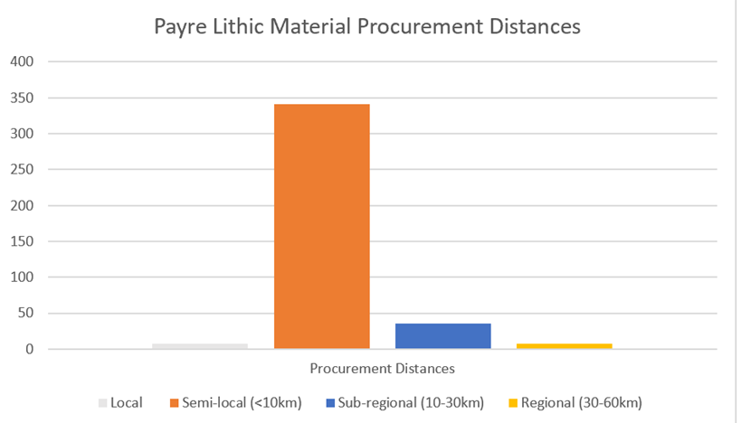
Figure 1: Payre (France) Procurement distances of lithic materials: data drawn from Moncel et al (2019)

In short, lithic transfer data is useful in giving us a direct connection with prehistoric people and their possible movement ranges. However, the data lacks a degree of complexity in the conclusions it affords us– hence the need to study isotopic and modern animal studies to help fill in the gaps and build on the lithic foundation.

2.2) Faunal Isotopic Studies

Another form of evidence with which we can attempt to decipher Neanderthal movement patterns is that of isotopic analysis. These analyses which, similar to lithic transfer analysis, draw on direct evidence from the past, can incorporate isotopic data directly drawn from Neanderthal remains, or data drawn from faunal remains. Thus, in the case of faunal isotopic data, making parallels, as with studies of modern animals, between faunal movements and Neanderthal movement. However, the distinction between the two is that faunal isotopic evidence is drawn directly from past animals, without the need to make assumptions about behaviours being consistent over time.

The principles on which isotopic studies relating to movement patterns are based are that organisms absorb isotopes at certain ratios throughout their lifetimes, with ratios matching their local environment and/or their food consumption (Hobson, K.A. 1999). In archaeology the tooth enamel is especially studied as teeth are sequentially formed and build up slowly throughout the lifetime of herbivores. Therefore, a time frame can be established with a possible seasonal/temporal basis for ratio patterns. Typically, strontium isotopes are the focus of these types of studies. However, others, such as oxygen and carbon, can be used.

A moderate number of studies incorporating both faunal and Neanderthal isotopic data have been undertaken. These studies highlight many of the advantages that come with using this data. For example, in the case of reindeer, a recent strontium, carbon and oxygen study (Price, et al, 2017) in Northern Germany was able to establish directionality of reindeer movement, suggesting that reindeer herds mostly follow an east-west movement through the region at the time. Furthermore, another strontium study of tooth enamel was able to give a crude idea of distances travelled and migration patterns of Bison and Reindeer, suggesting that Bison occupied a local range, while reindeer showed considerable seasonal migration patterns (Britton, et al, 2011).

It is clearly the case therefore that isotopic analysis of faunal remains can give us an understanding of movement issues, such as directionality, distances and migration patterns. However, it is also the case that these studies can be imprecise and crude – lacking an awareness of the intricacies of movement. It is also true that the number of these studies is limited in comparison to, for example, modern animal studies.

When it comes to Neanderthal isotopic studies, we have an opportunity to apply these same principles, but without the need to make parallels between faunal behaviour and Neanderthal behaviour. Rather, as with lithic transfer procurement, the data is directly connected to Neanderthal individuals themselves. Studies of this sort can be extremely useful in giving us a direct link to Neanderthal movement patterns. For example, at the site of Lakonis in Greece (Richard, et al, 2008), researchers were able to analyse strontium isotope ratios (Figure 2) from a 40,000 year old Neanderthal third molar and established that the individual must, due to the fact that the individual registered a different isotopic signature during a tooth growth stage which corresponded with the ages of 7 to 9 years old, have moved a considerable distance throughout their lifetime (at least in excess of 20km). Clearly, as with faunal isotopic studies, the conclusions drawn from this from of evidence can be illuminating.

Figure 2: Strontium isotope ratios of Neanderthal, rhino and deer enamel and dentine: Richard, et al, 2008: Figure 1

However, when it comes to Neanderthal isotopic studies, the same drawbacks apply in terms of imprecision, while the number of studies utilising this data is even more limited than with the faunal equivalents.

2.3) Modern Faunal Studies

Given the limitations associated with lithic transfer data and isotopic data, it is important to consider how we can supplement these sources of data with data drawn from modern animal studies. These studies incorporate an array of technique and methodologies, including the use of satellite telemetry, CRW (the correlated random walk computer model) (Bergman, et al, 2000), radio-tracking (Jedrzejewski, et al, 2001) and GPS tracking (Sylvatica and Hungrica, 2009).

Perhaps the greatest advantage with using this data is that the sheer volume of these studies outnumbers isotopic and lithic studies considerably. Researchers within the biological sciences have been able to construct a thorough understanding of the behaviour and movement patterns of many animal species, including red deer, reindeer, wolf and bison. Given the numerosity of studies, and the availability of “specimens” for present-day observation, researchers have been able to draw a wide array of conclusions with firm, quantitative data. For example, a Mediterranean study of radio-tracked red deer was able to determine that males had a home-range size 3-4 times that of females (Carranz, et al 1991). A study of bison in the North-western territories of Canada determined the daily activity of bison is characterised by alternation between resting and foraging phases (Larter and Gates, 1994). Furthermore, in regards to wolf, a Polish (Biolawezia Forest) study was able to quantitatively determine daily movement distances for adult females, concluding that winter movements tended to be greater than summer movements (Jedrzejewski, et al, 2001).

The intricacies and depth of the aforementioned data, encompassing an array of environments and climates, answering a considerable number of different behavioural and movement questions and incorporating a wide array of different techniques, would be difficult to determine simply based on archaeological resources. This therefore highlights the key advantage with incorporating modern faunal studies – the depth and abundance of studies.

There are, however, problems that come with drawing upon this data, particularly as a sole resource. These problems are, in part, a problem with the study of patterns in nature, while also linked solely with the use of modern analogues within the sphere of archaeology.

Firstly, modern day animal studies themselves have shown that animals within the same group – or even within the same species – do not always behave in the same way. This is especially true when put under different environmental and ecological pressures – though differences can occur regardless. For example, studies of European steppe bison have suggested that certain species such as Bison bison athabascae are non-migratory while other species such as Bison bonasus demonstrate migratory patterns within certain habitats – particularly mountainous regions (Hulien, et al, 2012). Therefore, based on this, we must be wary of making broad-based, sweeping conclusions (without qualification) about movement patterns given that nature is not always predictable. Building on this variability, it must also be true that making comparisons between modern day faunal behaviours and past faunal behaviours without assuming any room for error, or complementing these with direct archaeological evidence, would be wrong.

Regardless of this, however, it must be said that commonly occurring, repetitious patterns can often be noted in modern studies, particularly amongst certain groups of species. For example, red deer have been shown in modern animal studies to be consistent in their migration patterns (See Figure 3), displaying larger home-range sizes during autumn/winter months than summer months (Nahlik, et al, 2009). Similarly, it has long been noted that migrations to high-altitudes during summer months is commonly repetitious behaviour amongst cervids (Kropil, et al, 2015).

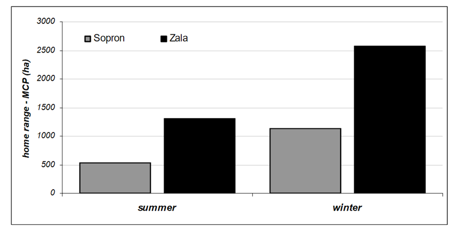
Figure 3: Home Range of hinds in Sopron and Zala by season: Nahlik, et al, 2009: Figure 1

Clearly, there is fundamentally a very strong advantage and disadvantage associated with using modern faunal studies within archaeology. The advantage is the wide array of studies with researchers drilling down into finer detail than is possible with lithic and isotopic data. However, the issue of variability and unpredictability within nature, and associated behaviours and movement patterns, does arise – particularly when applying the present to the past.

2.4) Literature Summary

The depth of data that can be drawn on in this study is relatively numerous. There have been a moderate number of studies which incorporate isotopic data, giving us a broad-based understanding of issues such as directionality and home-range sizes from a direct source. Similarly, lithic transfer data gives us a very direct connection with past peoples, with a start and end point to draw on. However, while these areas are accurate and direct, they are also lacking depth and precision. By drawing on modern faunal studies, we can address the question of precision, understanding the behaviours and movements of these species in much finer detail.

Chapter Three: Methodology

3.1 Materials

The types of sources, the species included, and the study locations incorporated in this dissertation will now be considered.

3.1.1 The Species Included

Four groups of faunal species have been studied. These are: red deer, bison, reindeer and wolf. These species were chosen, firstly, because they have a widespread geographic presence during the present day, and secondly, because they are associated with Neanderthal populations during the Middle Palaeolithic. Furthermore, the inclusion of herbivorous (red deer, reindeer and bison) and carnivorous (wolf) species allows us to make considerations based on likely prey, as well as the behaviour of potentially like-minded hunters.

3.1.2 Present-Day Distribution

All four of these species groups are presently extant. The present-day distribution of red deer can be seen in Figure 4. Distributions of a sample of existing bison herds can be seen in Figure 5. Distributions for European and North American wolves can be seen in Figures 6 and 7, respectively.

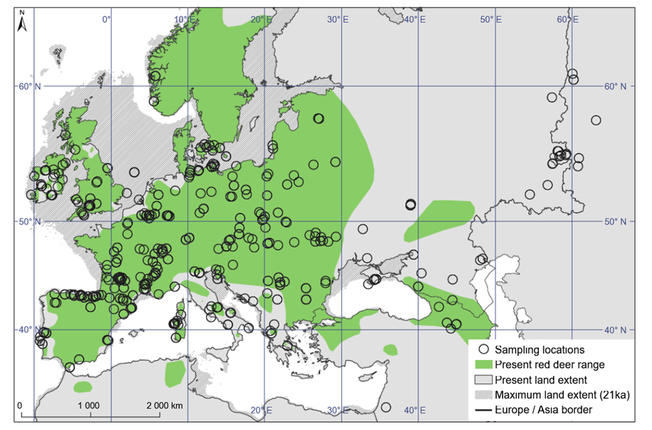
Figure 4: Present-day red deer range (green): Niedzialkowska, et al, 2020: Figure 1

Figure 5: Distribution of a sample of existing American bison herds: Sanderson, et al, 2008: Figure 1

Figure 6: Map of European wolf distribution: Stronen, et al, 2013: Figure 1

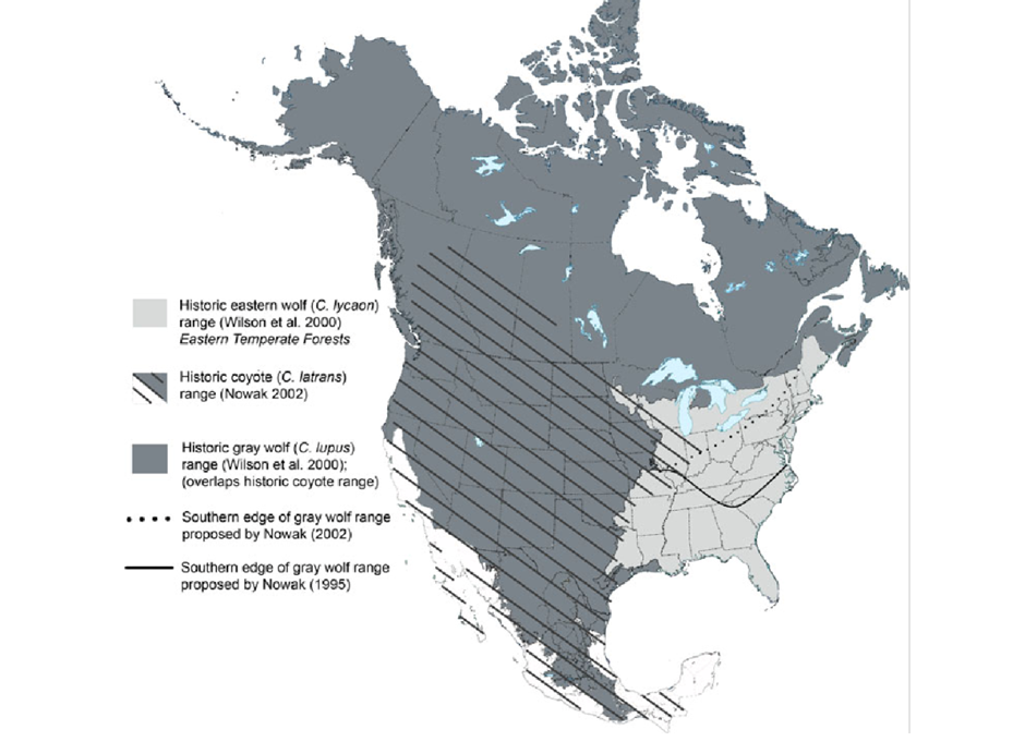
Figure 7: Map of wolf distribution in North America: Rutledge, et al, 2009: Figure 1

Most reindeer, meanwhile, have a northly distribution, with presence in North America (Wilson, et al, 2018) – mostly Canada – and in northern Asia (Anderson, 2006) and Europe (Burkhard and Muller, 2008).

3.1.3 Neanderthal-Faunal Associations

The Neanderthal associations with these four groups of species are clear. For example, a major study of 323 Neanderthal sites encompassing a range of European countries (Figure 8) covering MIS stages 7-3, suggests that bison (Bison Priscus), red deer (Cervus elaphus) and reindeer (Rangifer tarandus) are amongst the most commonly occurring (See Figure 9) in faunal assemblages (Patou-Mathis, 2000). Red deer show a consistently high presence, with greater than 60% representation in all MIS stages. Meanwhile, reindeer show greatest presence during glacial stages (MIS 7, MIS 5d-a, MIS 4 and MIS 3). Bison similarly are most prevalent during these glacial stages. However, they, unlike reindeer, show moderate prevalence (28.5%+) during all MIS stages. Overall, averages of all stages are: 78.5% for red deer, 45.5% for bison and 38.7% for reindeer.

Figure 8: Geographical locations of the countries considered in the work: Patou-Mathis, 2000:: Figure 1

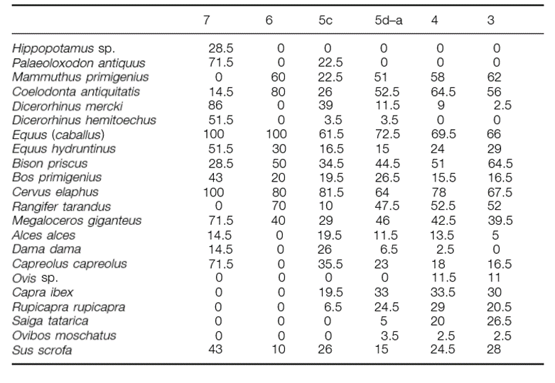
Figure 9: Representation of herbivore taxa related to isotopic stages (in per cent): Patou-Mathis: Table 5

Wolves meanwhile, were (as with Neanderthals) a Middle Palaeolithic predator (Germonpre, et al, 2009). Therefore, they are worth considering as a possible broad model for predator movement.

3.1.4) Sources

This dissertation aims to draw on as many sources as possible. The principle sources are journal articles from the biological sciences. However, for collection of the lithic and isotopic data, more traditionally archaeologically relevant sources have been drawn upon. Overall, the sources are highly cross-disciplinary.

3.1.5) Study Locations (Modern Faunal)

A total of 52 study locations have been used for determining the faunal model. These study locations are presented in Table 1, alongside their coordinates, Koppen-Geiger climatic classification and source. Locations for isotopic and lithic data are presented in Chapters Four and later in this chapter, respectively.

Location	Species	Latitude and Longitude	Koppen-Geiger Climatic Zone	Source
Israel, Negev Desert	Wolf	30.5⁰N, 34.9⁰E	BWh (hot desert)	Hefner & Geffen, 1999
Central Appenines, Italy	Wolf	42.5⁰N, 13.4⁰E	Csa (Mediterranean)	Mancinelli, et al, 2018
Croatia, Dalmatia	Wolf	43⁰N, 16.4⁰E	Csa (Mediterranean)	Kusak, et al, 2005
Poland, Bialowieza	Wolf	53⁰N, 24⁰E	Dfb (humid continental)	Okarma, et al, 1998
Slovakia, Caparthians	Wolf	49⁰N, 20.2⁰E	Dfb (humid continental)	Findo & Chovancova, 2004
Italy , Sirente Mountain range	Wolf	42.2⁰N, 13.6⁰E	Cfc (oceanic)	Ciucci & Boitani, 1997
Alaska Range	Wolf	63⁰N, -150.5⁰W	Dfc (subarctic)	Burch, et al, 2010
Scandinavian Peninsula	Wolf	62⁰N, 12.63⁰E	Dfc (subarctic)	Mattisson, et al, 2013
Canada, Yukon	Wolf	61.8⁰N, 132.5⁰W	Dfc (subarctic)	Hayes, et al, 2000
Alaska, Yukon Flats	Wolf	66.7⁰N, 145.7^0W	Dfc (subarctic)	Lake, et al, 2015
Poland – Bialowieza	Wolf	52.69⁰N, 23.85⁰E	Dfb (humid continental)	Jedrzejewski, et al, 2001
Alaska, Nelchina	Wolf	62⁰N, 146.8⁰W	Dfc (subarctic)	Burkholder, 1959
Spain, Monfrague National Park, Caceres	Red deer	39.8⁰N, 5.94⁰W	Csa (Mediterranean)	Pepin, et al, 2009
East Germany (Grafenwohr)	Red deer	49.85⁰N, 11.94⁰E	Dfb (humid continental)	Reinecke, et al, 2013
Central Germany	Red deer	51.55⁰N, 9.23⁰E	Dfb (humid continental)	Reinecke, et al, 2013
Hungary, Zala County	Red deer	46.6⁰N, 16.86⁰E	Dfb (humid continental)	Nahlik, et al, 2009
North Germany, Schleswig-Holstein	Red deer	55.01⁰N, 10.5⁰E	Cfb (oceanic)	Reinecke, et al, 2013
Italy, Tarvisio Forest	Red deer	46.3⁰N, 13.36⁰E	Cfb (oceanic)	Luccarini, et al, 2006
Hungary, Sorpon Mountains	Red deer	47.7⁰N, 16.5⁰E	Dfb (humid continental)	Nahlik, et al 2009
Italy, Susa Valley	Red deer	45.1⁰N, 6.53⁰E	Dfb (humid continental)	Luccarini, et al, 2006
Great Hungarian Plains	Red deer	47.3⁰N, 19.8⁰E	Dfb (humid continental)	Szemethy, et al, 2003
Slovakia, Kremnica	Red deer	48.7⁰N, 18.93⁰E	Dfb (humid continental)	Kropil, et al, 2014
Bulgaria, Balkans	Red deer	47.3⁰N, 25.1⁰E	Dfb (humid continental)	Zlatanova, et al, 2015
Saskatchewan	Reindeer	53⁰N, 160.5⁰W	Dfb (humid continental)	Wilson, et al, 2018
British Columbia, Maxhamish	Reindeer	58.2⁰N, 130⁰W	Dfc (subarctic)	Wilson, et al, 2018
Quebec, Charlevois	Reindeer	47.54⁰N, 70.6⁰W	Dfb (humid continental)	Wilson, et al,
Alberta, West side Athabasca	Reindeer	54.72⁰N, 113⁰W	Dfb (humid continental)	Wilson, et al, 2018
Alberta, East Side Athabasca	Reindeer	54.72⁰N, 113⁰W	Dfb (humid continental)	Wilson, et al, 2018
Ontario, Sydney	Reindeer	50.9⁰N, 93.9⁰W	Dfb (humid continental)	MNRF, 2014
Quebec, Manigougan	Reindeer	50.64⁰N, 68.75⁰W	Dfb (humid continental)	Wilson, et al, 2018
Ontario, Churchill	Reindeer	51.83⁰N, 92.83⁰W	Dfb (humid continental)	MNRF, 2014
Manitoba, Flintstone Lake	Reindeer	50.7⁰N, 95.3⁰W	Dfb (humid continental)	Wilson, et al, 2018
Ontario, Brightsand	Reindeer	50.24⁰N, 90.2⁰W	Dfc (subarctic)	MNRF, 2014
Ontario, Nipigon	Reindeer	50.21⁰N, 89⁰W	Dfc (subarctic)	MNRF, 2014
Ontario, Kinloch Lake	Reindeer	52⁰N, 91.2⁰W	Dfc (subarctic)	MNRF, 2014
Labador, Mealy Mountains	Reindeer	53.4⁰N, 59.5⁰W	Dfc (subarctic)	Wilson, et al, 2018
Alberta, Chinchaga	Reindeer	57.54⁰N, 119⁰W	Dfc (subarctic)	Wilson, et al, 2018
Ontario, Spirit	Reindeer	53.6⁰N, 92.6⁰W	Dfc (subarctic)	MNRF, 2014
Snake-Sahtahneh	Reindeer	56.17⁰N, 126.3⁰W	Dfc (subarctic)	Wilson, et al, 2018
Ontario, Berens	Reindeer	52⁰N, 94.3⁰W	Dfc (subarctic)	MNRF, 2014
NWT South	Reindeer	61.8⁰N, 118⁰W	Dfc (subarctic)	Wilson, et al, 2018
NWT North	Reindeer	68.5⁰N, 127⁰W	Dfc (subarctic)	Wilson, et al, 2018
Ontario, Pagwachian	Reindeer	49.7⁰N, 86.1⁰W	Dfc (subarctic)	Wilson, et al, 2018
Ontario, Ozhiski	Reindeer	52⁰N, 88.5⁰W	Dfc (subarctic)	Wilson, et al, 2018
Ontario, Kesegami	Reindeer	50.37⁰N, 80.28⁰W	Dfc (subarctic)	MNRF, 2014
Labrador, Lac Joseph	Reindeer	52.75⁰N, 65.31⁰W	Dfc (subarctic)	Wilson, et al, 2018
Labrador, Canada, Red Wine Mountains	Reindeer	54⁰N, 62⁰W	Dfc (subarctic)	Wilson, et al, 2018
Ontario, Missisa	Reindeer	52.9⁰N, 85.7⁰W	Dfc (subarctic)	MNRF, 2014
Canada, George River	Reindeer	59.4⁰N, 66.38⁰W	Dfc (subarctic)	Bergman, et al, 1999
Canada, Mink Lake	Bison	61.7⁰N, 117⁰W	Dfc (subarctic)	Larter & Gates, 1990
Osage County, Oklahoma	Bison	36.7⁰N, 96.4⁰W	Cfa (humid subtropical)	McMillan, et al, 2021
Comanche County, Oklahoma	Bison	34.35⁰N, 98⁰W	Cfa (humid subtropical)	McMillan, et al, 2021

Table 1: Summary of faunal modern-day faunal study locations, including the species group, location, coordinates, climatic zone and source

3.2) Methods
The methods for constructing the modern faunal model, incorporating direct faunal lithic data and testing against Neanderthal lithic data will be considered.

3.2.1) Modern Faunal Analysis – Determining Modern Day Movement Patterns

To determine the movement patterns of the four groups of species featured, a species-by-species analysis of a wide array of available data for movement patterns has been made based on the sources and locations noted above (Table 1). These movement patterns have been recorded in data sets, and tested against variables. The intention of this is to find broad-based patterns of movement for each species and for all species. Based on this the following questions, amongst other, can be answered:

Do all species show increases in home ranges as the climate becomes colder and more barren? How do home ranges vary based on individual climatic zones?
Do species show consistencies in terms of sexual difference in home ranges? (i.e do males/females roam further?). Similarly, are there consistencies based on season?

Answering these questions allows for the construction of qualitative and quantitative models of faunal movements with conclusions based on different variables. Having done this, the following question can be considered:

How does this model for movement compare with presently-available models/estimates for Neanderthal movements based on direct Neanderthal associations (i.e. lithics/isotopes)?

The methodological process for determining the answer to this question will be addressed later in this chapter.

3.2.2) Measures of Faunal Movement

Primarily, this study will consider quantitative data for home range sizes, due to its frequent occurrence in studies. However, the following further measures of movement have also been included:

Wolf

Daily movement distance
Daily movement speed

Red Deer

None

Bison

Average distance for movement “events”

Reindeer

4-day daily movement average

3.2.3) The Variables – Looking for Patterns in the Data

Home range sizes will be tested and considered based on a range of variables. These variables are as follows:

Latitude
Longitude
Koppen-Geiger climatic zone
Seasonality
Sex

The methodological processes for each of the variables are as follows:

3.2.4) Determining Latitude and longitude

For each faunal population shown in Table 1, latitudinal and longitudinal coordinates have been noted. Based on this, simple comparisons between latitude and home range sizes and longitude and home range sizes have been made.

3.2.5) Determining Climate

Latitude and longitude can, in many ways, be considered a proxy for climate. It is commonly known, for example, that the further north one travels from the equator, the colder it becomes. However, analysing solely based on these rudimentary comparisons misses the real subtleties of the climatic topography of the earth. For this reason, the true impact of climate on home ranges is not entirely visible based simply on latitudinal and longitudinal analysis. For example, there is not a completely strict correlation between latitude and climatic classification across the reindeer’s principal habitat (Canada). In this case, certain areas of high latitude (i.e. northern Alberta) have temperate continental climates, while certain areas of low latitude (i.e. parts of southern Ontario) have subarctic climates (See Figure 10). Therefore, koppen-Geiger climatic zones are a variable with which home ranges have been tested against.

Figure 10: Canadian Koppen-Geiger climatic distribution: Amani, et al, 2019: Figure 1

The worldwide climatic topography based on Koppen-Geiger classifications can be seen in Figure 11. Based on interpretations of Koppen-Geiger maps such as seen in Figure 10 and Figure 11, the following climatic distribution can be seen for study locations incorporating quantitative annual home range data for each group of species (Table 2). In total, five climatic zones are covered by these locations, with most (41 out of 48 of the home range study populations) of the faunal populations in humid continental or subarctic zones.

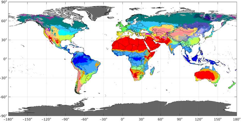
Figure 11: Koppen-Geiger world climatic map: Beck, et al, 2018: Figure 1

Climatic Zone	Wolf	Red Deer	Bison	Reindeer	Total
Humid continental (Dfb, Dsa, Dwb, Ddb, Dfa, Dwa)	2	8	0	8	18
Subarctic (Dfc, Dsc, Dsd, Dwc, Dwd, Dfd)	4	0	2	17	23
Mediterranean (Csa, Csb)	2	1	0	0	3
Oceanic climate (Cfb, Cwb, Cwc, Cfc)	1	2	0	0	3
Desert (BWh, BWk)	1	0	0	0	1
Total	10	11	2	25	48

Table 2: Number of studies that incorporate quantitative home range data for each Koppen-Geiger climatic zone: data drawn from sources noted in Table 1

3.2.6) Determining Seasonality and Sex

Some studies look at movement patters based on the seasons. For example, Findo and Chovancova (2004) include a spring to summer mean for home ranges of Slovakian wolves, alongside an autumn to winter mean and an annual yearly mean. Some studies also present this kind of consideration for other methods of discerning movement. For example, Wlodzimierz et al (2001) include monthly averages for daily movement distances – from which seasonal variations can be discerned. For this dissertation, seasonal data has simply been recorded and presented in graphical formats.

Similarly, some studies include differences between males and females. For example, Larter and Gates (1990) include home range averages for males and females in their study of Canadian wood bison. This is further illustrated by Nahlik et al (2009) in their study of Hungarian red deer home ranges and Zlatanova et al (2019) in their study of Bulgarian red deer home ranges. As with the variable of seasonality, this sex-based data has simply been recorded and presented graphically.

3.2.7) Bringing it all Together – Construction of Model

For the construction of the qualitative model, it was simply a case of noting the key conclusion for each variable (based on the species), firstly, in descriptive fashion in Chapter Five and, secondly, in a succinct table also in Chapter Five.

3.2.8) Isotopic Analysis

The conclusions present in the qualitative and quantitative models have been tested against isotopic data from the Middle Palaeolithic concerning the four groups of species. This data has been obtained from a total of five sources, incorporating strontium, oxygen and carbon-based data. The primary intent of this is to determine whether there are obvious differences between Middle Palaeolithic faunal populations and their modern-day counterparts. The number of relevant isotopic studies are, however, miniscule when compared with relevant modern faunal studies. Therefore, it is difficult to determine a significant amount from this data.

3.2.9) Incorporating Direct Neanderthal Evidence

The above methodological process has been used to create a model for faunal movements. However, this data must be tested against direct and indirect models for Neanderthal movement. In order to do this, lithic data has been drawn upon.

3.2.10) Lithic Comparisons – Determining Whether Faunal Trends Apply

The most prominent means by which archaeologists determine Neanderthal movement patterns is lithic procurement data. Lithic procurement is based on the idea that the original source of a lithic 23 material can be determined, and thus the distance between this source and where the lithic was found represents an estimate for the distance a Neanderthal population may have travelled. A number of studies, such as Feblot-Auugustins (1992) incorporate this method of analysis.

Given that it is impossible to determine differences based on sex and seasons, alongside the small geographic range of most of the lithic sites incorporated (thereby making latitudinal and longitudinal analysis less worthwhile), the variable of climate will be solely considered. This will be done in a similar way to the faunal side of this dissertation with an attempt to make comparisons between Koppen-Geiger climatic zones of the present and equivalent climatic zones in the Middle Palaeolithic.

3.2.11) Middle Palaeolithic Climatic Considerations

It is impossible to draw exact comparisons between Koppen-Geiger climatic zones of the present and likely geographic climate topography in the past. However, we can make broad-based estimates for regional climates in the Middle Palaeolithic for both the interglacial and glacial periods. The climatic estimates are as such:

3.2.12) Determining Interglacial Period Climatic Zones

During the Middle Palaeolithic, there were a number of interglacial periods (See Figure 12). During these interglacial periods, we can infer much the same climatic topography as today. This is illustrated in figure 13, which demonstrates the presence of vegetation commonly found in the present-day climatic zones – i.e. Mediterranean evergreen woodland in Spain and Italy, deciduous forest in central and eastern Europe and mixed conifer and boreal forest in Scandinavia.

For interglacial periods, therefore, the five climatic zones will be considered as follows:

Subarctic – Scandinavia
Humid continental – central and Eastern Europe
Oceanic – France and Britain
Mediterranean – Italy and Spain
Desert/semi desert – Africa and the Middle East

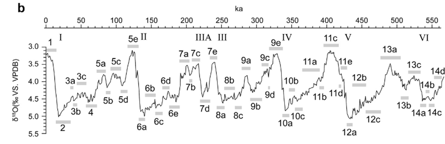
Figure 12: Marine isotope fluctuations in the Quaternary: Gibbard and Lewin, 2016: Figure 1

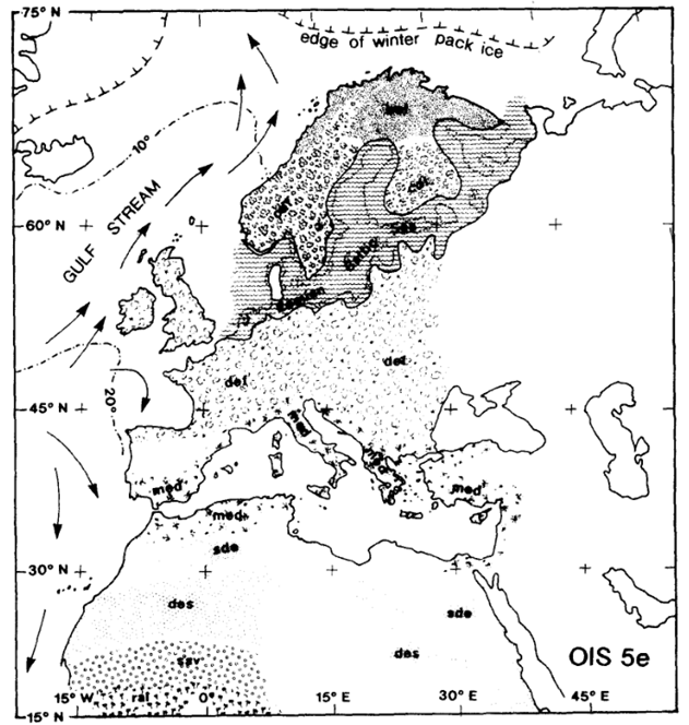
Figure 13: Sketch map of Europe during the optimum of the last interglacial: Van Andel and Tzedakis, 1996: Figure 9

3.2.13) Determining Glacial Period Climatic Zones

For glacial periods, the vegetational history (Figure 14), alongside the colder temperatures, suggests that most of Europe experienced subarctic conditions. This is exemplified in the greater presence of reindeer in Europe during this time (Patou-Mathis, 2000). The climatic zoning for glacial periods is thus as follows:

Subarctic- Europe above the alps
Humid continental – most of Europe below the alps
Mediterranean – small patches of Spain and Italy
Desert/semi-desert – Africa and the Middle East

Figure 14: Sketch map of Europe during the OIS 6 glacial: Van Andel and Tzedakis, 1996: Figure 9

Overall, the following sites (Table 3) have been drawn upon for the lithic analysis segment of this dissertation, with the determined climatic zone and source noted.

Location	Estimated Climatic zone	Source
Payre, France	Oceanic	Moncel, et al, 2019
Central Europe (40 Combined Sites)	Humid continental	Feblot-Augustins, 1992
Sabalyuk Cave, Poland	Humid continental	Ciesla, et al, 2018
Champ Grand, France (MIS 3)	Subarctic	Churchill, 2016
Raj Cave, Poland	Humid continental	Churchill, 2016
Le Rond de Saint-Arcons (MIS 3)	Subarctic	Churchill, 2016
Vaufrey, France (MIS 7-6)	Subarctic	Churchill, 2016
Baume Valley (MIS 5a)	Oceanic	Churchill, 2016

Table 3: Neanderthal lithic sites incorporated, alongside estimated climatic zone and source

3.2.14) Lithic-Based Home Range Calculations

Further to recording and presenting lithic procurement distances, home range estimates based on lithics will be included for a more like-for-like comparison with the faunal model.

Home range calculations have been made based on the idea that procurement distances tell us the maximum distance Neanderthals could have travelled from a particular point (where the lithic is found), and therefore this distance forms the radius of a circular home range estimate for Neanderthals. Therefore, in order to determine the area of the range, a simple πr² calculation is needed. For example, a procurement distance of 10km would be equivalent to a home range radius of 10km and, based on πr², a circular home range area of 314km². These types of estimates have already been undertaken by Churchill et al (2016), which will be incorporated.

It is important to note that the sample size is significantly smaller for the lithic procurement section of this study than the faunal movements section. This is partly a result of the unavailability of significant numbers of academic sources and the fact that this dissertation is primarily focused on the faunal perspective. As a result of this, the conclusions of the lithic analysis must be taken with more caution than the conclusions of the faunal analysis. Furthermore, faunal home ranges and lithic procurement are far from being a completely like-for-like comparison.

Chapter Four: Results

4.1) Predator Movement Patterns (Wolves)

To understand the movement patterns of Neanderthals, it is useful to consider the movement patterns of other predator species. The species Canis lupus (grey wolf) is a key predator species which was commonly present throughout the Middle Palaeolithic Neanderthal world (Germonpre, et al, 2009), while also having a broad distribution in the modern day (Corsi, et al, 1999; Mech, et al, 1988; Blanco, et al, 1992). As per the methods set out in Chapter Threee, a series of variables will be considered against modern-day movement patterns. Furthermore, considerations of carnivore dietary patterns drawn from direct palaeolithic isotopic and zooarchaeological evidence, including a further carnivore species (Canis diris), will be incorporated.

4.1.1) Home Range Sizes (Wolf)

The home range sizes of Canis lupus, from ten separate studies incorporating population data from ten separate locations, can be seen in Figure 15. Annual yearly home range sizes vary in these studies from just 34km² in the Negev desert in Israel, to 1608km² in the Yukon flats of Alaska. However, it should be noted that few studies of wolf home ranges have been undertaken at such a low latitude as the Negev desert and in none of the other studies do average annual home ranges fall below 100km².

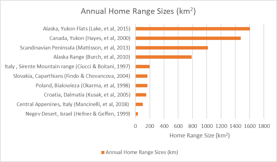
Figure 15: Annual yearly home range sizes of wolf populations from ten separate studies encompassing ten separate locations

^{4.1.2) Latitude and Climate (Wolf)}Clearly there is a high degree of variability in home range sizes. However, this variability corresponds reasonably with the latitudinal positioning of the populations studied. Figure 16 suggests that there is a correlation between latitude and home range size. In the case of wolves, home range seems to increase as northerly latitude increases, with a particularly sharp increase above 60⁰N. In fact, none of the home ranges below 55⁰N are greater than 200km², while the home ranges above 60⁰N are all higher than 700km² (most of them significantly so).

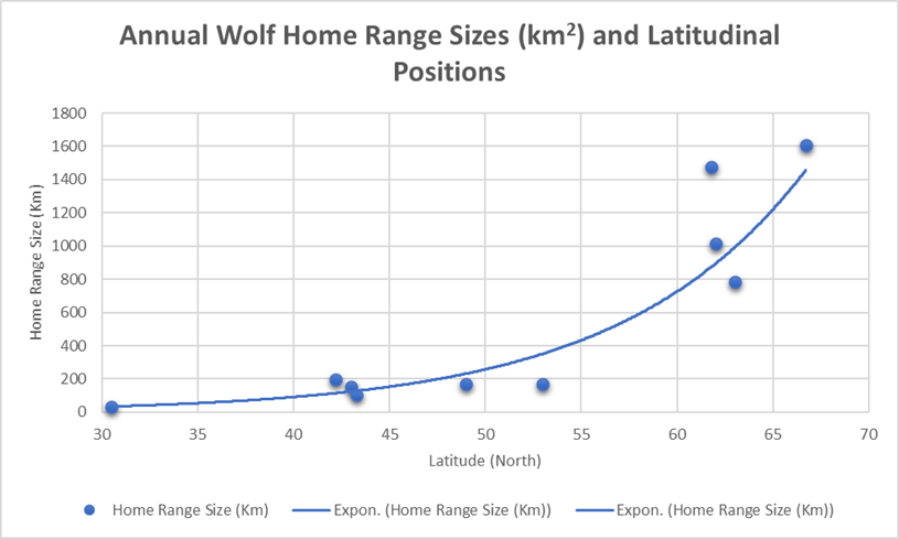
Figure 16: Annual home range sizes (km) from studies encompassing ten locations, with home ranges sizes directly compared with likely latitudinal position

The data can also be conveniently grouped according to climatic zones, as seen in Figure 17. This chart illustrates that there is not simply a linear increase in home ranges as northerly latitude increases (i.e., a certain degree of expansion for every degree moved north), but rather there is an expected range for broad climatic zones (See Table 4). There is an identifiable hot, deserted cluster (with a singular study suggesting a home range of 34km²), a mild cluster encompassing oceanic, Mediterranean and humid continental climates (ranging from 104km² to 197km²) and a subarctic cluster (ranging from 787km² to 1608km²). This is further illustrated in Figure 4, with averages for each climatic zone included.

Figure 17: Annual home range sizes (km) from studies encompassing ten locations, with home range sizes directly compared with latitudinal position and grouped climatically

Climatic Zones	Range	Average
Desert	34km²	34km²
Mediterranean	104-150.5km²	127.2km²
Oceanic	197km²	197km²
Humid continental	168-169km²	168.5km²
Subarctic	787-1608km²	1223km²

Table 4: Climatic zones featured in the ten wolf studies, with overall ranges in home range size, as well as averages, included

All of these findings suggests that wolf home ranges are moderately predictable and uniform, despite initial impressions from Figure 13. If knowledge of the location, latitude or climatic group is known, one could estimate the likely home range size of a population with some degree of certainty. It is possible that other Species, including Neanderthals, also display a similar relationship between home range size and latitude/climate. Thus, paleoclimatic/environmental data is a very important consideration for Neanderthal sites and populations.

Determining whether this pattern is replicable in other animal species, and could be applied to Neanderthals, is key to this dissertation.

4.1.3) Longitude (Wolf)There is longitudinal correlation with home ranges (Figure 18) – home ranges generally increase from west to east. However, it is also the case that the latitudinal distribution of wolves tends to increase from east to west.

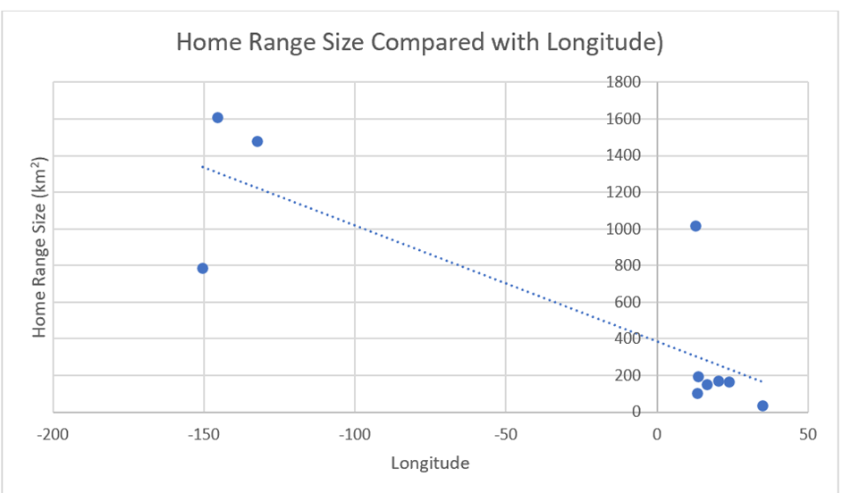
Figure 18: Wolf home range sizes from the ten study locations compared with longitude

4.1.4) Seasonality (Wolf)

Seasonally-based home range data seems to suggest larger home range sizes in the winter than in the summer (See Figures 19 and 20). This therefore means that wolves show predictable movement seasonally as well as annually. However, the smaller sample size should bring greater reason for caution.

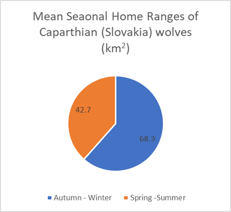
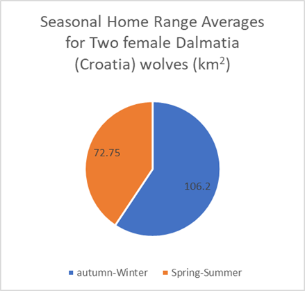
Figures 19 and 20: Mean seasonal home ranges of Carpathian (Slovakia) and Dalmatia (Croatia) wolves, categorized seasonally (Findo & Chovancova; Kusak, et al, 2005)

4.1.5) Daily Movement Distances (Wolf)It is important toconsider themovement patterns of wolves on a smaller timescale, looking at their daily movement distances and daily movement speeds. In the case of both, a smaller amount of data is available than home range sizes. However, some data is available, as per Figure 21. These three studies suggest a small degree of daily movement variability, with a range from 22.8km per day in the Bialowieza Forest in Poland (Wlodzimierz, et al, 2001) to 27.4km per day in the Sirente Mountains of Italy (Ciucci & Boitani, 1997). The average daily movement distance from these three studies is 25km.

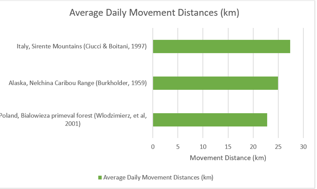
Figure 21: Average daily movement distances from three studies in three separate locations

4.1.6) Daily Movement and Latitude (Wolf)

It seems, based on these three studies, that latitude and climate have little to no bearing on daily movement distances. This is illustrated in Figure 22, which shows no meaningful trend.

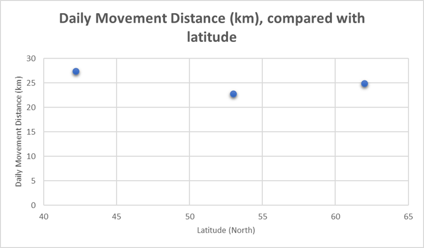
Figure 22: Daily movement distances of from three wolf studies (above), compared with latitude

4.1.7) Daily Movement and Seasonality (Wolf)

Only one identified study has seasonal data for daily movement distances (Jedrzejewski, et al, 2001). This study (Figure 23) suggests that wolves generally display greater daily movement distances during colder months than warmer months. Figure 24 illustrates the higher daily movements during winter months (24.4km) compared with summer months (19.7km). However, the largest months do not fall within these seasons, and are in fact in Spring (March) and Autumn (September, November).

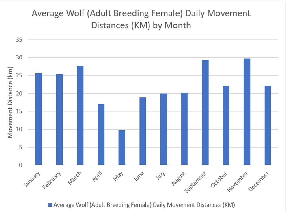
Figure 23: Average wolf daily movement distances categorized by month, drawn from a study of Bialowieza (Poland) wolves (Jedrzejewski, et al, 2001)

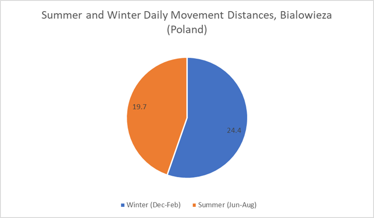
Figure 24: Summer and winter daily movement distances of Bialowieza (Poland) wolves (Jedrzejewski, et al, 2001)

4.1.8) Daily Movement Speeds (Wolf)

Only two studies have been identified which calculate wolf daily movement speeds. These studies are in the Bialowieza Forest in Poland (Wlozimierz, et al, 2001) and Sirente Mountains in Italy (Ciucci & Boitani). The movement speeds calculated are 2.3km/h and 2.5km/h, respectively. The average is 2.4km/h. it is difficult to state, based on two studies, whether movement speed is consistent across latitudes, climates, and seasons. More research is needed on wolf movement speeds to help answer these questions.

4.1.9) Human Impacts

A caveat that should be mentioned regarding these modern faunal studies is the involvement of humans in the lives of many of these populations. For example, in the Slovakian Carpathian population, the individuals dwell in a National park, potentially limiting their range use. In study areas such as the Italian Sirente Mountains (Ciucci & Boitani, 1997) and Israeli Negev desert, there is extensive human settlement. In fact, studies of the Negev desert wolves suggest that they spent an average of 52.3% of their time foraging in the vicinity of human settlement (Hefner & Geffen, 1999). Furthermore, the impact of humans on the wider ecology should also not be underestimated. Population declines of many big game animals have been noted throughout history, including bison (Flores, 1991), musk deer (Yang, et al, 2003) and reindeer (Vors & Boyce, 2009). It is not unreasonable, therefore, to assume human impacts on the resource availability of modern populations may impact upon their movement patterns. Indeed, all of these human factors could have an impact.

4.2) Predator Isotopic and Faunal Evidence

Direct isotopic evidence for palaeolithic wolf populations has been identified in two studies. Neither of these studies address movement directly. However, they address diet, which can give us an indication of the sorts of prey wolves were hunting or scavenging for.

The first of these studies focuses on specimens of the extinct dire wolf species Canis dirus from the La Brea tar pits in California. This study seems to suggest that dire wolves had varied diets (See Figure 25), incorporating primarily large herbivores, including bison, horse, mastodon, camel and sloth (Fox-Dobbs, et al, 2007). Furthermore, analysis of dire wolf morphology, including robust skulls and tooth breakage, suggests that they were well adapted to hunting or scavenging large prey (Binder, et al, 2002).

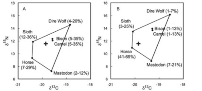
Figure 25: Mean dire wolf carbon and nitrogen values plotted with potential diet sources: Fox-Dobbs, et al, 2007: Figure 6

The second relevant study focuses on two palaeolithic sites. At the site of Goyet Cave in Belgium, the carbon and nitrogen values indicate that individuals (See Figure 26) G-7 and G-5 consumed horses most frequently, along with some horse-consumption evidence for individual G-1. Meanwhile, individuals G-8 and G-2 likely consumed both horse and bison (Germonpre, et al, 2009).

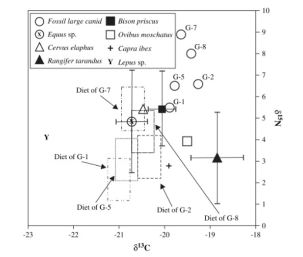
Figure 26: Carbon and nitrogen isotope signatures of fossil wolves and herbivores from Goyet Cave. Rectangular boxes represent possible isotopic values of average prey: Germonpre, et al, 2009: Figure 9

At the site of Trou du Frontal, two canid individuals were studied. The isotopic values are not consistent with any of the species the study focused on (See Figure 27), however the range of isotopic values for the first individual (TN-1) has been determined to be closest to that of red deer, while the range for the second individual (TN-2) is closest to that of aurochs (Bos primigenius) and bison (Bison priscus).

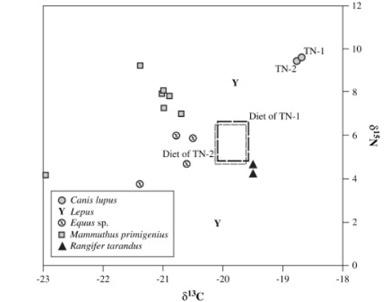
Figure 27: Carbon and nitrogen isotope signatures of fossil wolves from Trou des Nutons and contemporary herbivores. Rectangular boxes represent possible isotopic values of average prey consumed by the wolves: Germonpre, et al, 2009: Figure 7

Both of these studies suggest large prey consumption. This is consistent with modern populations of wolf, which have been found to consume large species such as deer (Potvin, et al, 1988), elk, moose (Popp, et al, 2018) and bison (Blackburn, et al, 2014). This, therefore, suggests that, firstly, wolves have had somewhat consistent dietary habitats over time and, secondly, greater credence is given to the idea that the movement patterns of large prey species are worth incorporating as they may have been somewhat in lockstep with predator movements.

4.3) Predator Results Conclusions

Overall, it is clear that there is some degree of predictability when it comes to the movement patterns of wolves. Home range correlates somewhat with latitude and longitude, while they show larger home ranges and movement distances during winter.

Direct evidence in the form of zooarchaeological and isotopic data suggests that wolves, from two species, had diets which included large prey. This is consistent with many modern populations, and suggests a connection is likely between the movements of large carnivores and large herbivores.

4.4) Prey Movement Patterns

Prey movement patterns are considered based on similar criteria as predator movement patterns so as to determine overlap between the two. Species of red deer, bison and reindeer will be considered in turn. All of these species are notably present at Middle Palaeolithic Neanderthal sites (Patou-Mathis, 2000).

4.5) Red Deer4.5.1) Home Ranges (Red Deer)

14 red deer (Cervus Elaphus) home ranges are shown in Figure 28. Red deer home ranges are typically presented in most studies in hectares rather than km². Thus, the original data (in ha) has been presented here, with a converted average for comparisons with other species later in the chapter. The data in Figure 28 includes examples of studies which include non-migratory, residential individuals. This data has been highlighted in orange. Most of the following analysis, however, will focus on migratory individuals.

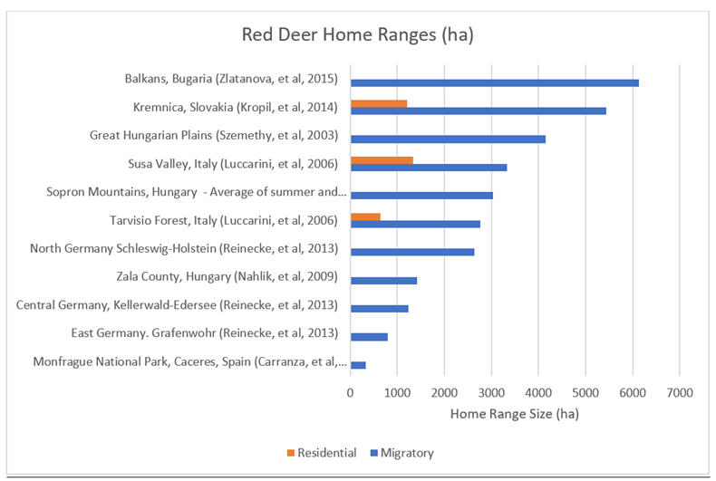
Figure 28: Red deer home ranges from 10 study locations

Red deer home ranges are, on average, significantly smaller than wolf home ranges. The average of wolf studies is 572km², compared with just 33.27km² for red deer. This is still true when comparing red deer home ranges with wolf home ranges in European temperate climates (See Table 5), however the difference is significantly smaller.

Climatic Zone	Migratory Red Deer Home Range Average (km²)	Wolf Home Range Average (km²)
Deserted	N/A	34km²
Mediterranean	3.37km²	127.2km²
Oceanic	27km²	197km²
Humid continental	31.9km²	168.5km²
Subarctic	N/A	1223km²

Table 5: Red deer home ranges, grouped climatically

4.5.2) Latitude and Longitude (Red Deer)

Unlike with wolves, little correlation can be seen between latitude and home range (See Figure 29. However, there a notable longitudinal correlation, with a west to east increase in home ranges (Figure 30).

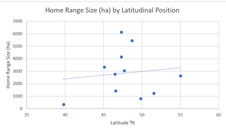
Figure 29: Home ranges of the 11 (above) red deer populations compared with their latitudinal position

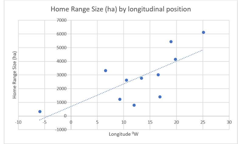
Figure 30: Home ranges of the 11 (above) red deer populations compared with their longitudinal position

4.5.3) Climate (Red Deer)

The red deer home ranges fall within three Koppen-Geiger climatic zones – Cfb (oceanic), Dfb (humid continental) and Csa (Mediterranean). In Figure 31, a sharp rise in home ranges from the Mediterranean zone to the oceanic zone can be seen, with a more modest rise into the humid continental zone.

Figure 31: Home ranges of the 11 (above) red deer populations, with averages calculated based on their climatic classification

4.5.4) Seasonality (Red Deer)

Red deer show partial consistency in their seasonally-based home range patterns. Obtainable statistics for seasonal home range are shown in Figure 32.

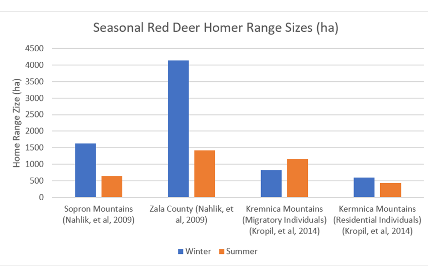
Figure 32: Seasonal-based home ranges for four red deer populations

The data from Figure 32 seems to suggest a consistently larger home range sizes during winter months. This is similarly observable in the home ranges of female red deer in three further sites in Germany (Figure 33). However, there is some variation evident in this data. Notably, the migratory Kremnica Mountain individuals display larger summer ranges, as do the males at the German sites shown in Figure 33. Similarly, data from the Tarvisio Forest and Susa Valley areas of Italy presents a very mixed picture, with stationary red deer showing little seasonal variation and migratory red deer showing large Autumn and Spring ranges and comparatively miniscule summer and winter ranges (Figure 34).

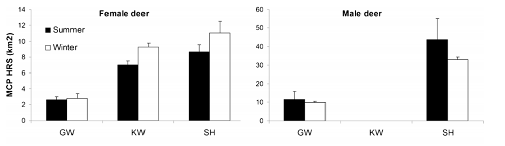
Figure 33: Seasonally based home ranges for male and female red deer at East (GW), North (SH) and Central (KW) German sites: Reinecke, et al, 2014: Figure 1

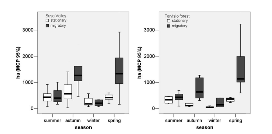
Figure 34: Seasonally based home ranges for stationary and migratory red deer populations at the Italian sites of Susa Valley and Tarvisio Forest: Luccarini, et al, 2006:Figure 2

Overall, therefore, larger winter home ranges are the predominant trend. However, there is notable variability.

4.5.5) Sex (Red Deer)A handful of studies give us annual home ranges based on sex. The results show a consistent pattern. Males within the same herd/region demonstrate larger home ranges than females (See Figure 35).

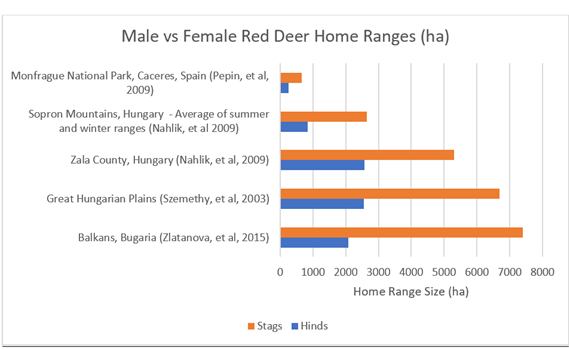
Figure 35: Home ranges of five red deer populations, with comparisons based on sex

4.6) Bison

Modern faunal data for bison, particularly of the quantitative kind, is limited. Therefore, the following analysis is less detailed and focuses on fewer variables than with the other species featured.

4.6.1) Home Ranges (Bison)

Home range data is sparse in modern bison faunal studies. However, one study with home range data for a Canadian (Mink Lake) bison population does exist – suggesting a home range size of 607km². This study falls within a subarctic Koppen-Geiger zone.

4.6.2) Sex (Bison)

This Mink Lake study has male and female-based home ranges. The study suggests (Figure 36) significantly greater ranges for female bison – this is obviously in stark contrast to red deer.

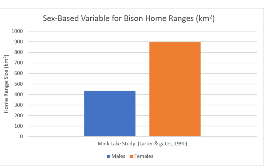
Figure 36: Sex-based differences in home ranges for the above Canadian Mink Lake population

4.6.3) Movement Distances (Seasonal) (Bison)

Data is available for average movement distances of bison during movement events at two sites in Oklahoma, USA. The data, in contrast with wolf daily movement distances, suggests greater movement during warmer seasons – particularly in the case of the site of Wichita Mountains (See Figure 37).

Figure 37: Seasonally based average movement distances of two Oklahoma bison populations: data drawn from McMillan, et al, 2021

4.7) Reindeer
Reindeer, another species with Neanderthal associations (Patou-Mathis, 2000), will now be considered.

4.7.1) Home Ranges (Reindeer)

The reindeer home ranges in Figure 38, all based on Canadian populations, range from 312km² to 8838 km². The average range is 1937km².

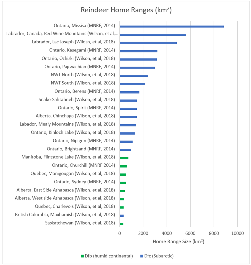
Figure 38: Home ranges (km²) for 25 populations of Canadian reindeer. Populations residing in humid continental areas have been highlighted in green, while those residing in subarctic areas are highlighted in blue

4.7.2) Latitude (Reindeer)Similarly to red deer, reindeer do not display the same kind of neat correlation based on latitude as wolves. There is a slight upward trend. However, there are many outliers (Figure 39).

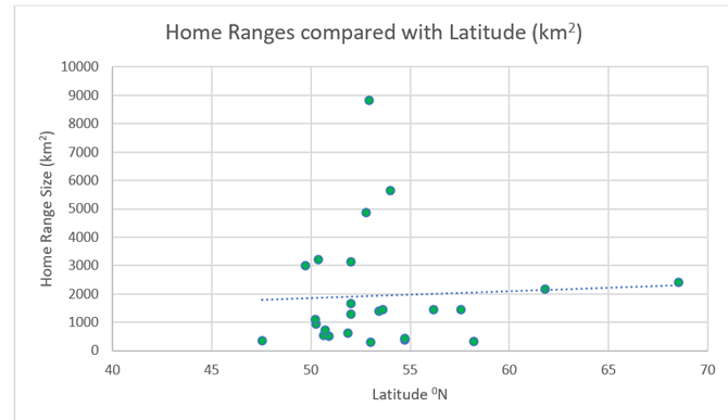
Figure 39: Home ranges of the above 25 populations of reindeer, compared with latitudinal position

4.7.3) Longitude (Reindeer)When it comes to longitude, there is slightly more corelation than with latitude – there is a general increase in home ranges moving from west to east. However, there are many clear exceptions to this rule (Figure 40).

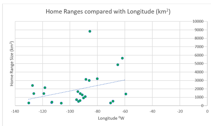
Figure 40: Home ranges of the above 25 populations of reindeer, compared with longitudinal position

4.7.4) Climate (Reindeer)
Broadly speaking, the distribution of reindeer falls within two Koppen-Geiger climatic zones – Dfb, (humid continental) and Dfc (subarctic). Here we can see much greater correlation than with latitude or longitude (See Figure 41). Subarctic home ranges are significantly larger than humid continental home ranges. In fact, 8 of the 9 smallest home ranges are humid continental climates, while the top 16 are all subarctic.

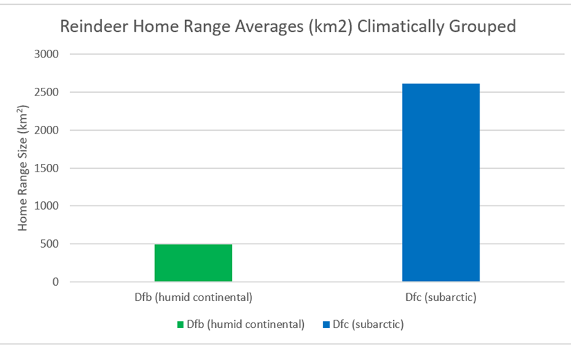
Figure 41: Home ranges of the above 25 populations of reindeer, climatically grouped

4.7.5) 4-Day Movement Distances – Seasonally Based (Reindeer)

One particular study, based on a Canadian (George River) reindeer population, incorporates averages for 4-day movement distances (Bergman, et al , 1999). The study suggests that movement distances of reindeer are significantly reduced during winter months and are consistent throughout the rest of the year (Figure 42).

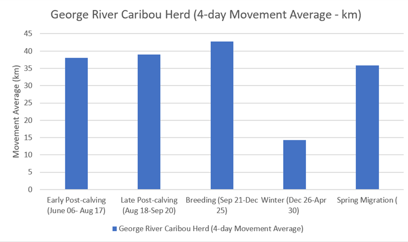
Figure 42: 4-day movement averages of a Canadian reindeer population: data drawn from Bergman et al (1999)

4.8) Prey Conclusions

Clearly, there are differences between these prey species – with seasonal, sex-based and latitudinal and longitudinal differences. Similarly, there are differences in terms of the typical home range sizes. However, as with wolf, there is overlap amongst all in terms of patterns of increase corresponding with climate.

4.9) Cross-Species Combined Analysis

Having looked at these four group of species in isolation, it is now worthwhile to combine and contrast (where applicable) cross-species data patterns.

4.9.1) Overall Home Ranges (Combined)

It is clear based on comparisons of the four groups of species (See Figure 43) that reindeer display the largest total home range sizes. Wolf and bison sit somewhere in the middle, while red deer consistently demonstrate the smallest home ranges. This is shown numerically in Table 6, which also displays numerical data for home rage averages for all the species according to Koppen-Geiger climatic classification.

Figure 43: Combined averages for total home ranges (km²) of red deer, wolf, bison and reindeer

Climatic Zone	Migratory Red Deer Home Range Average (km²)	Wolf Home Range Average (km²)	Bison Home Range Average (km²)	Reindeer Home Range Average (km²)	Average of all
Desert	N/A	34km²	N/A	N/A	34km²
Mediterranean	3.77km²	127.2km²	N/A	N/A	65.3km²
Oceanic	27km²	197km²	N/A	N/A	112km²
Humid Continental	31.94km²	168.5km²	N/A	492.2km²	230.9km²
Subarctic	N/A	1222km²	607km²	2616km²	1482km²
Total Home Range Average	28.44km²	571km²	607km²	1937km²

Table 6: Data set for home ranges of each group of species, averaged according to the Koppen-Climatic zone that they fall in. Combined averages are all presented for each climatic zone, alongside numerical averages for non-variable-based total home ranges for each group of species

4.9.2) Climate and Home Ranges (Combined)

When making considerations based on climate, we can see a relatively consistent pattern (Figure 44). Home ranges gradually increase as such: desert, Mediterranean, oceanic and humid continental. There is then a significant increase moving into subarctic conditions. These patterns can be seen with all species. The sole exception is wolf, which displays a greater range for oceanic over humid continental. However, this case should not be taken with too much credence as the oceanic wolf range is based on one solitary study.

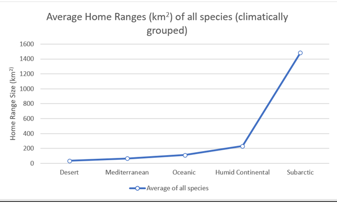
Figure 44: Combined averages for all species, grouped according to climatic zone

4.9.3) Latitude and Home Ranges (Combined)As can be seen from Figure 45, home range sizes for red deer, bison and wolf are similar for given latitudes (though wolf tends to track above the rest). However, when reindeer home ranges are added in (See Figure 46), there are a greater number of outliers between 50-55⁰N.

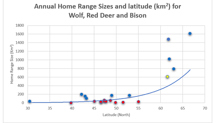
Figure 45: Ranges for wolf (blue), red deer (red) and bison (yellow) compared with latitude

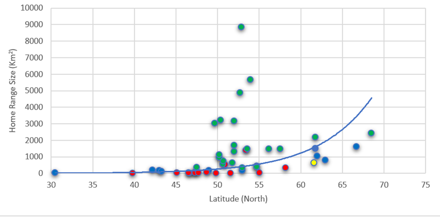
Figure 46: Ranges for wolf (blue), red deer (red), reindeer (green) and bison (yellow) compared with latitude

4.9.4) Seasonality, Sex and Home Ranges (Combined)
Cross-species patterns cannot be drawn based on sex and seasonality. There are strong patterns that do exists – however these are inter-species patterns rather than cross-species.

4.10) Faunal Isotopic Data (Prey Species)

As with wolf, direct evidence for past movements of the prey species exists in the form of isotopic data. The data seems to support the conclusion that reindeer display greater home ranges than bison. This is clear in Figure 47, with data from the Middle Palaeolithic site of Jonzac (France) showing bison strontium isotope values consistent with a local range (Britton, et al, 2011).

Figure 47: Sequential strontium data from reindeer and bison enamel: Britton, et al, 2011: Figure 3

Similarly, Julien et al (2012) suggest that bison occupied a limited range, with carbon values for all individuals consistent of a C3 steppe/grassland environment. This is illustrated in Figure 48, with most of the strontium isotope values for the 26 bison individuals falling within the expected narrow range.

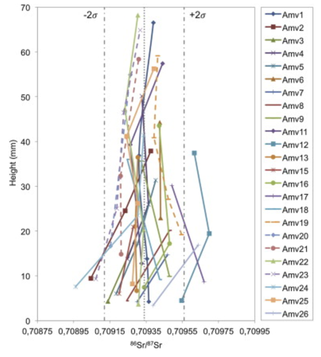
Figure 48: Enamel intra-individual variations of strontium values for Amrovievka bison: Julien, et al, 2012: Figure 4

Isotopic data from the Palaeolithic with a relevance to movement patterns of red deer was seemingly not available for this section.

4.11) Lithic Results
A brief analysis of some lithic procurement results will be presented here in Chapter Four. Discussion as to likely home range estimates from these results and correlation with the faunal model, will be undertaken in Chapter Five. Analysis based only on the variable of climate and longitude (broad east-west differences) will be undertaken here. Specifically, the focus will be on Western European lithic procurement distances and Eastern European lithic procurement distances, as these regions have received the most attention by archaeologists. The characterisation of the climatic conditions of different areas during different periods of the Middle Palaeolithic has been set out in Chapter Three.

4.11.1) Western European (Oceanic) Lithics

Oceanic procurement strategies, here characterized as procurement west of Germany during interglacial periods, suggests low levels of regional sourcing. Most studies suggest that lithics within these regions are typically highly “local.” This is shown in Figure 49, with regional/local procurement ratios at the site of Payre in France.

Figure 49: Lithic materials from the site Payre (France) based on percentage of local and regional sourcing; data drawn from Moncel et al (2019)

4.11.2) Central European (Humid Continental) Lithics

A major study of 40 sites across central Europe gives contrasting results from the above oceanic studies (Feblot-Augustins, 1993). As Figure 50 illustrates, an average of 53% of the lithics at these sites were found to be sourced more than 20km from where they were found. Clearly, there is evidence for Neanderthal range expansion moving into a likely more characteristics humid continental climate. This pattern of greater procurement distances in Central Europe (in comparison to Western and Northern Europe) is commonly recognised within archaeology (Churchill, et al, 2016), with some transfers in excess of 300km known in the late Middle palaeolithic of Central Europe (Dusseldorp, 2009).

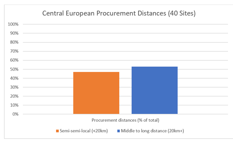
Figure 50: Lithic materials from 40 Central European Middle Palaeolithic sites based on percentage of local-semi-local and middle-long-distance sourcing: data drawn from Feblot-Augustins (1992)

Though the above study seems to suggest quite large procurement distances, there is variation. For example, at the Sabalyuk cave site in the Polish Western Carpathians (Ciesla, et al, 2018), only 17% of lithics were from regional sources (much lower than 53%).

4.11.3) Lithic Conclusions

Though there is some variation, there does seem to be evidence for an increase in lithic procurement distances moving from west to east, which may correspond with a likely move from an oceanic to humid continental climate.

Chapter Five: Discussion5.1) Conclusions – Establishing the Faunal Model

Short variable-by-variable summaries of the results for all species will now be made. These summaries form the basis for the qualitative model, which has been constructed in table form. Reasons for the evident variable-based patterns will be discussed, alongside the usefulness of the conclusions for each variable. The summaries below will therefore cover three key questions:

Are there patterns in the data?
Why do these patterns appear?
How useful/applicable are these conclusions?

5.1.1) Latitude and Longitude Conclusions

Regarding latitude, wolves displayed the clearest correlation with home range sizes. The one study below 30⁰N suggested a home range of just 34km². Meanwhile, everything from 40 – 55⁰N fell within a range of 100-200km², while everything above 60⁰N was higher than 750km². In contrast, red deer and reindeer showed very little, if any, correlation with latitude. It is worth, noting however, that this may have more to do with the current distribution of these species than any other factor. It is, perhaps, easier to see clearer latitudinal correlation when a species (such as wolves) covers vastly different portions of the world with more disparate temperatures, environments and climates.

Longitudinal analysis suggests a general increase in home ranges from east to west in wolves, west to east in reindeer and west to east in red deer.

The latitudinal and longitudinal correlations with home range that are present are likely the result of differences in climate (i.e. a general cooling moving northwards), resource availability and environment. Studies suggest that animals adapt their movements based on resource availability (Pellerin, et al, 2010) – which may include increased home ranges as resources become more scarce, subsequently requiring larger ranges to find. The above latitudinal and longitudinal patterns are useful in terms of understanding Neanderthal movement, in that they give a general sense of likely changes in home range based on the coordinates of a given Neanderthal population. However, these differences are only obviously clear when comparing vastly different latitudes and longitudes.

5.1.2) Climate Conclusions

Analysis undertaken based on Koppen-Geiger climatic zones provides for a finer-scale assessment of the impacts of climate, resource availability and environment, and subsequently produced more consistent results than analysis based on latitude and longitude. The combined faunal home ranges saw moderate expansion corresponding with the following pattern: desert (34km²), Mediterranean (65km²), oceanic (112km²), humid continental (231km²). There is then a large increase in home ranges moving into subarctic climatic conditions (1482km²).

As with longitude and latitude, the resource availability of different climatic zones may be determining home range sizes.

In this study, we can see consistent correlation across the 48 sites with home range data that have been incorporated. Therefore, given this consistency, it would not be unreasonable to assume that Neanderthal home ranges would correlate in a similar fashion. Therefore, this climatic data is a vitally important aspect of the faunal model and will be a key consideration in tests against Neanderthal lithic data later in this chapter.

5.1.3) Seasonality Conclusions

There is not the same extent of cross-species correlation between seasonality and home range as there is climate. Therefore, a universal rule for seasonality and animal movement could not be ascertained. However, there is correlation within the species groups themselves. For example, wolves show consistently higher home ranges and daily movement distances during winter months. This is also true of red deer, while bison show small ranges during inter and reindeer show small 4-day movement distances during winter.

Due to the existence of these inter-species patterns, rather than cross-species patterns, the model is only useful for applying to Neanderthal populations if corresponding dietary/faunal hunting data is available.

5.1.4) Sex-Based Conclusions

As with seasonality, sex-based differences vary by species. there are some observable inter-species patterns. In the case of red deer, males had larger average home ranges than females, while with bison the opposite was the case.

Differences based on sex may be useful in terms of helping to predict the types of prey that Neanderthals may have hunted. For example, in the case of red deer, it is probable that hinds would have been preferred over stags due to their smaller ranges – making them easier to track.

5.1.5) Qualitative Model (Table summary)

The above conclusions have been summarised in Table 7. This is the qualitative faunal model.

Variable	Wolf	Red deer	Reindeer	Bison	Cross-Species Conclusions
Overall Home Ranges (Non-Variable-Based)	Moderate sized combined home range – similar to bison	Small combined home range -by far the smallest	Large combined home range – by far the largest	Moderate sized combined home range (though lack of extensive data)	Combined home ranges very species dependent. Average from smallest to largest: red deer, wolf, bison, reindeer.
Latitude	Increased home range with latitude (south to north)	Little Correlation with Latitude (though with scattered and inconsistent northerly increase)	Little correlation with latitude (though with a scattered and inconsistent northerly increase)	N/A (lack of data)	General increase in latitude moving northwards (though only especially clear with wolves)
Longitude	Increase from west to east	Increase from west to east	Some correlation – east to west	N/A Lack of data	Regionally dependent increases
Seasonality	Larger home range and daily movement distances during winter months	Larger winter home ranges most common (with some exceptions)	4-day movement distances lowest during winter – consistent rest of the year	Average movement distances greatest during summer – lowest during winter.	Species-dependent and dependent on movement measure
Sex	N/A (Lack of data)	Males have significantly larger home ranges	N/A (lack of data)	Larger female home ranges	Species dependent
Climate	From smallest to largest home range: desert, Mediterranean, humid continental, oceanic, subarctic.	From smallest to largest home range: Mediterranean, oceanic, humid continental.	From smallest to largest home range: humid continental, subarctic.	N/A (lack of data – though the available subarctic ranges larger than combined averages of over climatic zones)	Consistent combined pattern of increase: desert, Mediterranean, humid continental, oceanic, subarctic

Table 7: Qualitative summaries of the faunal data, based on the variables set out

5.2 – Incorporating Faunal Isotopic Data

The model must now be tested against faunal isotopic data from the Middle Palaeolithic. This helps to determine whether there are notable differences between modern day animals and their palaeolithic equivalents.

There is some notable correlation here. For example, reindeer were shown, as in the modern faunal model, to have isotopic values most consistent with widespread migration. Similarly, bison ranges were shown to be smaller – also consistent with the modern-day faunal data. Regarding wolf, there is a suggestion that they pursued large herbivorous prey such as red deer and bison, further supporting the assumption that they would likely have had movement patterns in common with, firstly, key prey species and, secondly, Neanderthals – who also show associations with these species (Patou-Mathis, 2000). Overall, therefore, the isotopic data supports the validity and value of the faunal model that has been constructed.

However, the number of studies focusing on isotopic concentrations amongst Middle Palaeolithic fauna are limited, while the conclusions that can be drawn from them are very broad (i.e. the general landscape/diet, very approximate migration sizes etc) and non-specific. Therefore, faunal isotopic data does not add a huge amount to our understanding of animal movement and thus demonstrates, firstly, the value of the modern-day faunal model and, secondly, the need for more research on Palaeolithic faunal isotopes.

5.2.1) Testing the Model – How Does it Compare with Existing Lithic Data?

The conclusions of the faunal model will now be considered against Neanderthal lithic data.

5.2.2) Lithic Discussion – Climate

As per chapter Four, lithic procurement data suggests larger home ranges in Central European sites (corresponding with a humid continental climate – as set out in Chapter Three) than Western Europe (corresponding with an oceanic climate). This is illustrated in figure 51, which shows the numbers of regionally procured materials found in the Feblot-Augustin (1992) study of 40 Central European sites, and at the Western European site of Payre (France) (Moncel, et al, 2019).

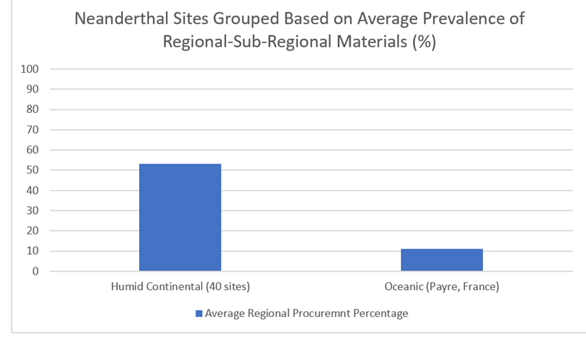
Figure 51: Comparisons between number of regionally procured materials in the Feblot-Augustin (1992) study the Moncel et al (2019)

5.2.3) Conversions to Home Range Size

As per the method set out in chapter 3, lithic data for Central Europe (Feblot-Augustins, 1992) and Payre, France (Moncel, et l, 2019) has been converted into home range sizes based on the most commonly occurring procurement distances in a sample. These estimates have been combined with available lithic-based home range estimates from Churchill (2016). Based on these conversions, a more like-for-like comparison with faunal data can be made.

The first estimate (for Central Europe) takes 20km as a threshold for procurement distance – given that a majority of lithics from this area are from a regional 20km source (Feblot-Augustins, 1992). Based on this, a home range of 1256km² has been ascertained. Similarly, given that the overwhelming majority of lithic materials form the Moncel et al (2019) study are from a local or semi-local source (represent 10km or less), a maximum home range of 314km²has been ascertained. Based on Churchill et al (2016), the following existing home range estimates from a range of sites encompassing a range of MIS periods have been added to these two estimates (See Figure 52).

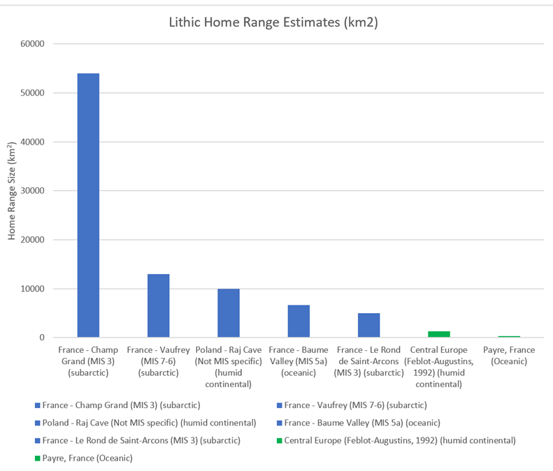
Figure 52: Estimated home ranges based on Feblot-Austins (1992) and Moncel et al (2019) in green, compared with existing home range estimates from Churchill et al (2016). This MIS period and corresponding estimate of climatic zone are stated.

These estimates are clearly larger than most of those in the modern faunal model – and also the new estimates made based on Feblot-Augustins (1992) and Moncel et al (2019). Overall, however, if averages are calculated for the above home ranges based on estimated climates, a near identical pattern arises as with the faunal model (See Figure 53). The combined faunal averages for these three climatic zones have been presented alongside (Figure 54) for clarity. Clearly, the rate of increase moving through the climatic zones is very similar.

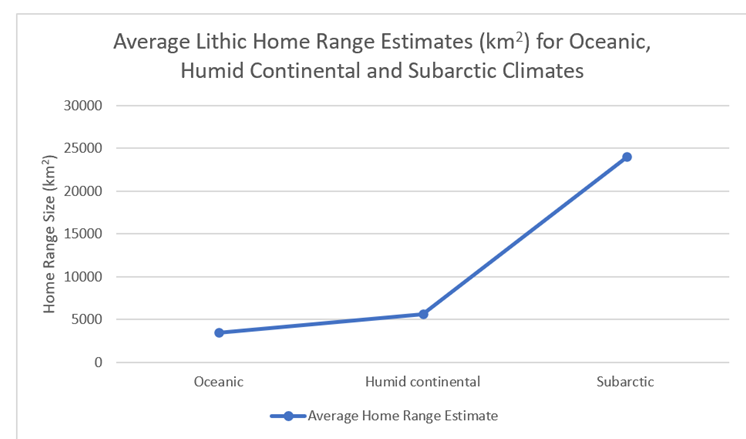
Figure 53: Climate-based averages of the lithic home range estimates presented in Figure 53

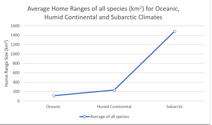
Figure 54: Home range averages from all species in the faunal model, grouped according to oceanic, humid continental and subarctic climates

5.2.4) Lithic Comparison Conclusions

Overall, the lithic data suggests very similar rates of increase in home range sizes across the climatic zones. However, the raw numbers for estimated home ranges based on lithic data are significantly greater than those suggested by the faunal model.

There are a few possible reasons for this. Firstly, these home range sizes may suggest that Neanderthal group sizes were large, with a subsequent requirement for more food. Secondly, it may be the case that stone tools were kept by Neanderthal individuals for significantly longer than the annual yearly period for the faunal home ranges. Therefore, the home ranges present above may be the cumulative ranges of Neanderthal individuals over significantly longer than 1-year periods. Furthermore, there could have been transfer between individuals and groups, further inflating the distances travelled. Thirdly, the climate, ecology and resource availability during the Middle Palaeolithic may have been significantly different than it is today – regardless of whether it was an interglacial period or not.

5.3) Neanderthal Isotopic data

Another direct source of evidence for Neanderthal movements is Neanderthal isotopic data. However, the study set out in Chapter Two is the only study with this data that could be found – with the data suggesting that the individual studied travelled 20km throughout their lifetime (Richards, et al, 2008).

Chapter Six: Conclusion

It is important to conclude this dissertation by setting out the answers to the key questions below.

6.1) How successful is the faunal model

Overall, the faunal model has been successful in drawing upon a very wide range of sources from the biological sciences and finding key patterns – both cross-species patterns and inter-species patterns. It is clear that the Koppen-Geiger climatic zone variable displays the most consistent, cross-species correlation. Meanwhile, the sex-based and seasonal-based variables display clear inter-species correlation (though some species lake the necessary modern data for these variables), while latitude and longitude show some correlation but with plenty of outliers and inconsistency – particularly regarding red deer and reindeer with their smaller (than wolf) geographic ranges.

Furthermore, the isotopic data supports many of the conclusions, such as larger reindeer ranges – though it is hindered by a lack of research and specificity.

6.2) Does the Faunal Model Fit with Existing Neanderthal Data?

Though the faunal model could only realistically be tested against one variable (climate), there is correlation with this in one sense – procurement distances clearly increase moving from the warmer (oceanic/Mediterranean) climates to the colder (humid continental/subarctic) climates. In fact, the rates of increase are very similar. However, the estimated home ranges based on lithic materials are significantly larger based on supposedly equivalent ranges.

6.3) What Research Need to be Undertaken in the Future?

Firstly, research into the above three potential reasons for the lithic disparity needs to be undertaken. Secondly, due to time constraints, this dissertation could not draw upon all possible variables (e.g. elevation, population-specific human impact etc). Therefore, further research is needed based on more variables. Thirdly, further research is needed on both faunal and Neanderthal (movement-relevant) isotopic analysis.

6.4) Final Thoughts

In summary, this project represents (as far as is known) the most authoritative analysis of the modern-day movement patterns of key Neanderthal predator and prey species. The faunal model can provide us with likely estimates for movement variables which could not be discerned based solely on lithic data (such as seasonality and sex), while also enhancing our understanding of the impact of climate on home ranges.

Furthermore, this research is equally important in terms of the findings when incorporating lithic data. Firstly, the equally consistent climate-based patterns of increase give credence to the faunal model, and suggest that patterns present in animals correlate, at least in this case, with hominins. However, beyond this, the stark difference in the raw numbers (with greater Neanderthal home ranges estimated from lithics) challenges us to rethink our understanding of the extent of Neanderthal movement and the nature of lithic procurement and transfer.

Bibliography

Amani, M., Mahdavi, S., Afshar, m., Brisco, B., Huang, W., Mirzadeh, S.M.J., White, L., Banks, S., Montgomery, J., Hopkinson, C., (2019) Canadian Wetland Inventory using Google Earth Engine: The First Map and Preliminary Results. Remote Sensing 11(7), 1-20

Anderson, D.G., (2006) Is Siberian Reindeer Herding in Crisis? Living with Reindeer Fifteen Years After the End of State Socialism. Nomadic Peoples 10(2), 87-104

Bergman, C.M., Schaefer, J.A., Luttich, S.N., (2000) Caribou movement as a correlated random walk. Oecologia 123 (3) 364-374

Blackburn, J.K., Asher, V., Stokke, S., Hunter, D.L., Alexander, K.A., (2014) Dances with Anthrax: Wolves (Canis lupus) Kill Anthrax Bacteremic Plains Bison (Bison bison bison) in Southwestern Montana. Journal of Wildlife Diseases 50(2), 393-396

Binder, W.J., Thompson, E.N., Van Valkenburgh, B., (2002) Temporal variation in tooth fracture among Rancho La Brea dire wolves. Journal of Vertebrate Palaeontology 22, 423-428.

Blanco, J.C., Reig, S., Cuesta, L.L., (1992) Distribution, status and conservation problems of the wolf Canis lupus in Spain. Biological Conservation 60(2), 73-80

Britton, K., Grimes, V., Niven, L., Steele, T.E., McPherron, S., Soressi, M., Kelly, T.E., Jaubert, J., Hublin, J.J., Richards, M.P., (2011) Strontium isotope evidence for migration in late Pleistocene Rangifer: Implications for Neanderthal hunting strategies at the Middle Palaeolithic site of Jonzac, France. Journal of Human Evloution 61(2), 176-185

Burch, J.W., Adams, L.G., Follmann, E.H., Rexstad, E.A., (2010) Evaluation of wolf density estimation from radiotelemetry data. Wildlife Society Bulletin 33(4), 1225-1236

Burkhard, B., Muller, F., (2008) Indicating human-environmental system properties: Case study northern Fenno-Scandinavian reindeer herding. Ecological Indicators 8(6), 828-840

Burkholder, B.L., (1959) Movements and Behaviour of a Wolf Pack in Alaska. The Journal of Wildlife Management 23(1), 1-11

Carranza, J., J.Hidalgo de Trucios, S., Medina, R., Valencia, J., Delgado, J., (1991) Space use by red deer in a Mediterranean ecosystem as determined by radio-tracking. Applied Animal Behaviour Science 30(3), 363-371

Churchill, S.E., Walker, C.S., Schwartz, A.M., (2016) Home-Range Size in Large-Bodied Carnivores as a Model for Predicting Neandertal Territory Size. Evolutionary Anthropology 25, 117-123

Ciesla, M., (2018) How far did they go? : exotic stone raw materials occurrence at the Middle Palaeolithic sites : case studies of sites from Western Carpathian Mts. Acta Archaeologica Carpathica 53, 7-28

Ciucci, P., Boitani, L., Francisci, F., Andreoli, G., (2009) Home Range, activity and movements of a wolf pack in central Italy. Journal of Zoology 243(4), 803-819

Corsi, F., Duprè, E., Boitani, L., (2008) A Large‐Scale Model of Wolf Distribution in Italy for Conservation Planning. Conservation Biology 13(1), 150-159

Dusseldorp, G.L., (2009) A View to a kill: Investigating Middle Palaeolithic subsistence using an Optimal Foraging perspective. 1^st ed. Leiden: Sidestone Press.

Féblot-Augustins, J., (1992) Mobility Strategies in the Late Middle Palaeolithic of Central Europe and Western Europe: Elements of Stability and Variability. Journal of Anthropological Archaeology 12(3), 211-265

Fox-Dobbs, K., Bump, J.K., Peterson, R.O., Fox, D.L., Koch, P.L., (2007) Carnivore-specific stable isotope variables and variation in the foraging ecology of modern and ancient wolf populations: case studies from Isle Royale, Minnesota, and La Brea. Canadian Journal of Zoology 84(4), 1-20

Flores, D., (1991) Bison Ecology and Bison Diplomacy: The Southern Plains from 1800 to 1850. The Journal of American History 78(2), 465-485

Findo, S., Chovancova, B., (2004) Home range sizes of two wolf pack in the Slovak Carpathians. Folia Zoologica 53(1), 17-26

Germonpré, M., Sablin, M.V., Stevens, R.E., Hedges, R E.M., Hofreiter, M., Stiller, M., Després, V.R., (2009) Fossil dogs and wolves from Palaeolithic sites in Belgium, the Ukraine and Russia: osteometry, ancient DNA and stable isotopes. Journal of Archaeological Science 36(2), 473-490

Gibbard, P.L., Lewin, J., (2016) Partitioning the Quaternary. Quaternary Science Reviews 151, 127-139

Hansen, B, B., Aanes, R., Saether, B.E., (2008) Partial seasonal migration in high-arctic Svalbard reindeer (Rangifer tarandus platyrhynchus). Canadian Journal of Zoology 88 (12), 1202-1209

Hayes, R.D., Harestad, A.S., (2000) Demography of a recovering wolf population in the Yukon. Canadian Journal of Zoology 78(1), 36-48

Hefner, R., Geffen, E., (1999) Group Size and Home Range of the Arabian Wolf (Canis lupus) in Southern Israel. Journal of Mammalogy 80(2), 611-619

Hobson, K.A., (1999) Tracing origins and migration of wildlife using stable isotopes: a review. Oecologia 120 (3), 314-326

Hulien, M.A., Bocherens, H., Burkea, A., Drucker, D.G., Patou-Mathis, M., Krotova, O., Péan, S., (2012) Were European steppe bison migratory? 18O, 13C and Sr intra-tooth isotopic variations applied to a palaeoethological reconstruction. Quaternary International 271 (31), 106-119

Jedrzejewski, W., Schmidt, K., Theuerkauf, J., Jedrzejewska, B., Okarma, H., (2001) Daily movements and territory use by radio-collared wolves (Canis lupus) in Bialowieza Primeval Forest in Poland. Canadian Journal of Zoology 79 (11), 1993-2004

Julien, M.A., Bocherens, H., Burke, A., Drucker, D.G., Patou-Mathis, M., Krotova, O., Pean, S., (2012) Were European steppe bison migratory? 18O, 13C and Sr intra-tooth isotopic variations applied to a palaeoethological reconstruction. Quaternary International 271, 106-119

Kropil, R., Smolko, P., Garaj, P., (2015) Home range and migration patterns of male red deer Cervus elaphus in Western Carpathians. European Journal of Wildlife Research 61, 63-72

Kusak, J., Skrbinsek, A.M., Huber, D., (2005) Home ranges, movements, and activity of wolves (Canis lupus) in the Dalmatian part of Dinarids, Croatia. European Journal of Wildlife Research 51(4), 254-262

Larter, N.C., Gates, C.C., (1990) Home Ranges of Wood Bison in an Expanding Population. Journal of Mammalogy 71(4), 604-607

Mancinelli, S., Boitani, L., Ciucci, P., (2018) Determinants of home range size and space use patterns in a protected wolf (Canis lupus) population in the central Apennines, Italy. Canadian Journal of Zoology 96(8), 828-838

Mattisson, J., Sand, H., Wabakken, P., Gervasi, V., Liberg, O., Linnell, J., Rune, G., Pedersen, H.C., (2013) Home range size variation in a recovering wolf population: evaluating the effect of environmental, demographic, and social factors. Oecologia 173(3), 813-815

Mech, L.D., Fritts, S.H., Radde, G.L., Paul, W.J., (1988) Wolf distribution and road density in Minnesota. Wildlife Society Bulletin 16(1), 85-87

MNRF (2014) Integrated Range Assessment for Woodland Caribou and their Habitat. Ministry of Natural Resources and Forestry.

Moncel, M.H., Fernandes, P., Wilmes, M., James, H., Grun, R., (2019) Rocks, teeth, and tools: New insights into early Neanderthal mobility strategies in South-Eastern France from lithic reconstructions and strontium isotope analysis. PLOS One 14(4), 1-30

Nahlik, A., Sandor, G., Tari, T., Kiraly, G., (2009) Space Use and Activity Patterns of Red Deer in a Highly Forested and in a Patchy Forest-Agricultural Habitat. Acta Silvatica 5, 109-118

Nielzialkowska, M., Doan, K., Gorny, M., Sykut, M., Stefaniak, K., Piotrowska, N., Jedrzejewska, B., Ridush, B., Pawelczyk, Mackiewicz, P., Schmolcke, U., Kosintsev., P., Makowiecki., Charniauski., M., Krasnodebski, D., Rannamae, E., Saarma, U., Arakelyan, M., Manaseryan, N., Titov, V.V., Hulva, P., Balasescu, A., Fyfe, R., Woodbridge, J., Trantalidou, K., Dimitrijevic, V., Kovalchuk, O., Wilczynski, J., Obada, T., Lipecki, ., Arabey, A., Stankovic, A., (2020) Winter temperature and forest cover have shaped red deer distribution in Europe and the Ural Mountains since the Late Pleistocene. Journal of Biogeography 48, 147-159

Jedrzejewski, W., Schmidt, K., Theuerkauf, J., Jedrzejewska, B., Okarma, H., (2001) Daily movements and territory use by radio-collared wolves (Canis lupus) in Bialowieza Primeval Forest in Poland. Canadian Journal of Zoology 79 (11), 1993-2004

Kropil, R., Smolko, P., Gara, G., (2014) Home range and migration patterns of male red deer Cervus elaphusin Western Carpathians. European Journal of Wildlife Research 61 (1), 63-72

Larter, N.C., Gates, C.C., (1994) Home-Range Size of Wood Bison: Effects of Age, Sex, and Forage Availability. Journal of mammalogy 75(1), 142-149

Lake, B.C., Caikoski, J.R., Bertram, M.R., (2015) Wolf (Canis lupus) Winter Density and Territory Size in a Low Biomass Moose (Alces alces) System 68(1), 62-68

Luccarini, S., Mauri, L., Apollonio, M., Lamberti, P., Ciuti, S., (2006) Red Deer (“Cervus elaphus”) Spatial Use in the Italian Alps : Home Range Patterns, Seasonal Migrations, and Effect of Snow and Winter Feeding. Ethology, Ecology & Evolution 18, 127-145

Moncell, M.H., Fernandes, P., Willmes, M., James, H., Rainer, G., (2019) Rocks, teeth, and tools: New insights into early Neanderthal mobility strategies in South-Eastern France from lithic reconstructions and strontium isotope analysis. PLoS ONE 14(4), 1-30

Okarma, H., Jȩdrzejewski, W., Schmidt, K., Śnieżko, S., Bunevich, A.N., Jȩdrzejewska, B., (1998) Home Ranges of Wolves in Białowieża Primeval Forest, Poland, Compared with Other Eurasian Populations. Journal of Mammalogy 79(3), 842-852

Pellerin, M., Calenge, C., Said, S., Gaillard, J.M., Fritz, H., Duancan, P., Laere, G.V., (2010) Habitat use by female western roe deer (Capreolus capreolus): influence of resource availability on habitat selection in two contrasting years. Canadian Journal of Zoology 88(11), 1-21

Potvin, F., Jolicoeur, H., Huot, J., (1988) Wolf diet and prey selectivity during two periods for deer in Quebec: decline versus expansion. Canadian Journal of Zoology 66(6), 1-15

Popp, J.N., Hamr, J., Larkin, J.L., Mallory, F.F., (2018) Black bear (Ursus americanus) and wolf (Canis spp.) summer diet composition and ungulate prey selectivity in Ontario, Canada. Mammal Rezearch 63, 433-441

Price, T.P., Meiggs, D., Weber, M.J., Pike-Tay, A., (2017) The migration of Late Pleistocene reindeer: isotopic evidence from northern Europe. Archaeological and anthropological sciences 9, 371-294

Reinecke, H., Leinen, L., Thiben, I., Meibner, M., Herzog, S., Schutz, S., Kiffner, C., (2013) Home range size estimates of red deer in Germany: environmental, individual and methodological correlates. European Journal of Wildlife Research 60, 237-247

Richards, M., Harvatia, K., Grimes, V., Smith, C., Smith, T.,Hublin, J., Karkanas, P., Panagopoulouc., (2008) Strontium isotope evidence of Neanderthal mobility at the site of Lakonis, Greece using laser-ablation PIMMS. Journal of Archaeological Science 35 (5), 1251-1256

Rutledge, L.Y., Bos, K.I., Pearce, R., White, B., (2009) Genetic and morphometric analysis of sixteenth century Canis skull fragments: implications for historic eastern and gray wolf distribution in North America. Conservation Genetics 11, 1273-1281

Sanderson, E.W., Redford, K.H., Weber, B., Aune, K., Baldes, D., Berger, J., Carter, D., Curtin, Charles., Derr, J., Dobrott, S., Fearn, E., Fleener, C., Forrest, S., Gerlack, C., Gates, C.C., Gross, J.E., Gogan, P., Grassel, S., Hilty, J.A., Jensen, M., Kunkel, K., Lammers, D., List, R., Minkowski, K., Olson, T., Pague, C., Robertson, P.B., Stephenson, B., (2008) The Ecological Future of the North American Bison: Conceiving Long-Term, Large-Scale Conservation of Wildlife. Conservation Biology 22(2), 252-266

Stronen, A.V., Drzejewska, B.J., Pertoldi, C., Demontis, D., Randi, E., Niedziałkowska, M., Pilot, M Sidorovich, V.E., Dykyy, I., Kusak, J., Tsingarska, E.,, Kojola, I., Karamanlidis, A.A., Ornicans, A., Lobkov, V.A., Dumenko, V., Czarnomskal, S.D., (2013) North-South Differentiation and a Region of HighDiversity in European Wolves (Canis lupus). Plos One 8(10), 1-9

Szemethy, L., Matrai, K., Katona, K., Orosz, S., (2003) Seasonal home range shift of red deer hinds, Cervus elaphus: are there feeding reasons?. Folia Zoologica 52(3), 249-258

Van-Andel, T.H., Tzedakis, P.C., (1996) Palaeolithic landscapes of Europe and environs, 150,000-25,000 years ago: An overview. Quaternary Science Reviews 15(5), 481-500

Vors, L.S., Boyce, M.S., (2009) Global declines of caribou and reindeer. Global Change Biology 15(11), 2626-2633

Wilson, K.S., Pond, B.A., Brown, G.S., Schaefer, J.A., (2018) The biogeography of home range size of woodland caribou Rangifer tarandus caribou. Diversity and Distributions 25(2), 205-216

Yang, Q., Meng, X., Xia, L., Feng, Z., (2003) Conservation status and causes of decline of musk deer (Moschus spp.) in China. Biological Conservation 109(3), 333-342

Zlatanova, D., Popova, E., Ahmed, A., Stepanov, I., Andreev, R., Genov, P., (2019) Red deer on the move: home range size and mobility in Bulgaria. Ecologica Montenegrina 23, 47-59

Dissertation